By the end of this chapter, students should be able to:
describe mathematical finance as the study of prices, cash flows, portfolios, uncertainty, and information;
distinguish prices, payoffs, simple returns, log returns, and portfolio values;
explain why arbitrage is a mathematical inconsistency in a financial model;
represent one-period asset payoffs as vectors and portfolios as linear combinations;
connect no-arbitrage pricing with linear algebra, probability, and discounting;
explain the difference between the real-world probability measure and the pricing probability measure;
understand the role of models: useful approximations, not exact descriptions of markets.
Mathematical finance begins with a simple question: what is a fair price today for a future uncertain cash flow?
The answer is not just a formula. It requires a model of uncertainty, a model of information, and a precise rule describing what trading strategies are allowed.
4.2 1.1 Why Mathematical Finance?
A financial asset has a price today and an uncertain value in the future. A derivative is a contract whose payoff depends on one or more underlying assets. A portfolio is a collection of positions in assets. Mathematical finance studies these objects using probability, linear algebra, optimization, stochastic processes, and numerical computation.
The central mathematical problem is this:
Given a future payoff, determine its present value under assumptions that exclude arbitrage.
For example, a European call option with strike \(K\) and maturity \(T\) pays
\[
(S_T-K)^+ = \max(S_T-K,0)
\]
at time \(T\). Its value today depends on the possible future values of \(S_T\), the interest rate, the market information, and whether the payoff can be replicated by trading other assets.
This book develops the mathematical ideas behind such questions. We begin in discrete time, where the main ideas are transparent. Later chapters move to Brownian motion, stochastic calculus, Black–Scholes theory, interest-rate models, risk measures, and portfolio optimization.
4.3 1.2 Prices, Payoffs, and Returns
Let \(S_t\) denote the price of an asset at time \(t\). In a deterministic setting, \(S_t\) is just a number. In a stochastic model, \(S_t\) is a random variable because future prices are uncertain.
4.3.1 Simple return
The simple return from time \(t\) to time \(t+1\) is
\[
R_{t+1}=\frac{S_{t+1}-S_t}{S_t}.
\]
Equivalently,
\[
S_{t+1}=S_t(1+R_{t+1}).
\]
The simple return measures relative gain or loss. If \(S_t=100\) and \(S_{t+1}=108\), then \(R_{t+1}=0.08\).
4.3.2 Gross return
The gross return is
\[
G_{t+1}=1+R_{t+1}=\frac{S_{t+1}}{S_t}.
\]
Gross returns multiply naturally over time:
\[
\frac{S_T}{S_0}=G_1G_2\cdots G_T.
\]
4.3.3 Log return
The log return is
\[
r_{t+1}=\log \frac{S_{t+1}}{S_t}.
\]
Log returns add naturally over time:
\[
\log\frac{S_T}{S_0}=r_1+r_2+\cdots+r_T.
\]
This additive property is one reason log returns are common in probability models and statistical estimation.
Definition 1.1 (Price process). A price process is a sequence of random variables
\[
S_0,S_1,\ldots,S_T,
\]
where \(S_t\) represents the price of an asset at time \(t\). The value \(S_0\) is usually known at time \(0\), while \(S_1,\ldots,S_T\) may be random.
Remark. Simple returns are natural for portfolio accounting. Log returns are natural for probability modeling. They are close when returns are small because
\[
\log(1+x)\approx x
\]
for small \(x\).
4.4 1.3 Riskless Asset and Discounting
A riskless asset, often called a bank account or money-market account, grows at a known rate. In a one-period model with interest rate \(r\), one dollar invested at time \(0\) becomes \(1+r\) dollars at time \(1\).
Let
\[
B_0=1, \qquad B_1=1+r.
\]
If a deterministic cash flow \(X\) is received at time \(1\), its present value is
\[
\frac{X}{1+r}.
\]
More generally, if a riskless bank account satisfies
\[
B_t=(1+r)^t,
\]
then the discounted value of a price process \(S_t\) is
\[
\widetilde S_t=\frac{S_t}{B_t}.
\]
Discounting converts future dollars into time-\(0\) dollars. Many pricing formulas are simplest when written in terms of discounted values.
Definition 1.2 (Discounted price). Given a riskless account \(B_t>0\), the discounted price of an asset \(S_t\) is
\[
\widetilde S_t=\frac{S_t}{B_t}.
\]
4.5 1.4 States of the World and Payoff Vectors
In a one-period model, uncertainty can be represented by a finite set of possible states:
This is the first major connection between finance and linear algebra:
Future cash flows are vectors; portfolios form linear combinations of payoff vectors.
Suppose there are \(d\) traded assets. Let \(S_0^j\) be the time-\(0\) price of asset \(j\), and let \(S_1^j(\omega_i)\) be its time-\(1\) payoff in state \(\omega_i\). A portfolio is a vector
\[
\theta=(\theta_1,\ldots,\theta_d)^\top,
\]
where \(\theta_j\) is the number of units held in asset \(j\).
A portfolio describes holdings in assets. In a one-period model, a portfolio is chosen at time \(0\) and produces a payoff at time \(1\). In a multi-period model, the portfolio may be adjusted over time.
A trading strategy is self-financing if all changes in the portfolio are paid for by selling and buying assets within the portfolio, with no external cash added or removed after the initial investment.
In discrete time, if \(\theta_t\) denotes the holdings during the period \((t,t+1]\), then the portfolio value is
\[
V_t=\theta_t\cdot S_t.
\]
The self-financing condition says that changes in wealth come only from price changes:
\[
V_{t+1}-V_t=\theta_t\cdot(S_{t+1}-S_t).
\]
This condition matters because pricing by replication only makes sense when the replicating strategy does not secretly inject extra money.
Definition 1.3 (Self-financing strategy). A trading strategy is self-financing if, after the initial portfolio is formed, all future changes in portfolio holdings are financed entirely by reallocating wealth among the traded assets.
4.7 1.6 Arbitrage
Arbitrage is the mathematical expression of a free lunch. It is a trading strategy with no possible loss, no initial cost, and positive gain in at least one state.
Definition 1.4 (Arbitrage in a one-period model). A portfolio \(\theta\) is an arbitrage if
\[
V_0(\theta)\le 0,
\]
\[
V_1(\theta,\omega)\ge 0
\quad \text{for all }\omega\in\Omega,
\]
and
\[
V_1(\theta,\omega)>0
\quad \text{for at least one }\omega\in\Omega.
\]
A model with arbitrage is internally inconsistent for pricing. If a payoff can be obtained for two different prices, then buying the cheaper version and selling the more expensive version produces a riskless profit.
No-arbitrage is not the statement that real markets never have mispricings. Rather, it is a modeling principle: in a liquid competitive market, large obvious arbitrages should not persist. Therefore a mathematical pricing model should not contain arbitrage opportunities as structural features.
4.8 1.7 A First One-Period Model
Consider a one-period model with two possible states: up and down.
At time \(0\), a stock has price
\[
S_0=100.
\]
At time \(1\), it can be
\[
S_1(u)=120,\qquad S_1(d)=80.
\]
The riskless asset grows from
\[
B_0=1
\]
to
\[
B_1=1.05.
\]
A European call option with strike \(K=100\) has payoff
\[
C_1=(S_1-K)^+.
\]
Thus
\[
C_1(u)=20,\qquad C_1(d)=0.
\]
We ask: what should \(C_0\) be?
4.8.1 Replication
Try to replicate the option using \(\Delta\) shares of stock and \(b\) dollars in the bank account at time \(0\). The time-\(1\) value of this portfolio is
\[
\Delta S_1 + b(1.05).
\]
To replicate the call payoff, solve
\[
120\Delta+1.05b=20,
\]
\[
80\Delta+1.05b=0.
\]
Subtracting the second equation from the first gives
\[
40\Delta=20,
\]
so
\[
\Delta=\frac12.
\]
Substituting into the second equation gives
\[
80\cdot \frac12+1.05b=0,
\]
so
\[
b=-\frac{40}{1.05}.
\]
Therefore the time-\(0\) cost of the replicating portfolio is
The no-arbitrage price of the call is approximately \(11.9048\).
Example 1.1 (Pricing by replication). The option payoff \((20,0)\) can be written as a linear combination of the stock payoff \((120,80)\) and the bond payoff \((1.05,1.05)\):
Thus the option price must equal the same linear combination of today’s prices:
\[
C_0=\frac12(100)-\frac{40}{1.05}.
\]
4.9 1.8 Risk-Neutral Probability
The same price can be written as a discounted expected payoff, but not necessarily under the real-world probability.
Let \(q\) be the probability of the up state under a new probability measure \(\mathbb Q\). We choose \(q\) so that the discounted stock price is a martingale:
Definition 1.5 (Risk-neutral probability in a one-period binomial model). The risk-neutral probability \(q\) is the probability under which the discounted stock price has no drift:
Equivalently, if \(S_1(u)=uS_0\) and \(S_1(d)=dS_0\), then
\[
q=\frac{(1+r)-d}{u-d}.
\]
Remark. The risk-neutral probability is not introduced because investors are risk-neutral. It is introduced because no-arbitrage prices can often be written as discounted expectations under a special probability measure. This measure is a pricing tool.
4.10 1.9 Physical Probability Versus Pricing Probability
There are two different probability measures that students must keep separate.
The physical probability measure, often denoted by \(\mathbb P\), describes the statistical behavior of the market. It is used for estimation, forecasting, simulation, and risk management.
The risk-neutral probability measure, often denoted by \(\mathbb Q\), is used for pricing. Under \(\mathbb Q\), discounted traded asset prices are martingales.
In general,
\[
\mathbb P\ne \mathbb Q.
\]
A common beginner mistake is to price an option by taking the expected payoff under the real-world probability and then discounting. That is usually not correct. The correct no-arbitrage pricing formula uses the pricing measure:
The real-world measure may assign a higher probability to the up state because investors expect the stock to grow. The pricing measure adjusts probabilities so that expected discounted gains of traded assets vanish.
4.11 1.10 No-Arbitrage as Linear Algebra
In a finite one-period model, no-arbitrage has a clean geometric interpretation.
Let \(p\in\mathbb R^d\) be the vector of time-\(0\) asset prices, and let \(A\in\mathbb R^{m\times d}\) be the matrix of time-\(1\) payoffs. A portfolio \(\theta\in\mathbb R^d\) has initial cost
\[
p\cdot \theta
\]
and payoff
\[
A\theta.
\]
An arbitrage exists if there is a vector \(\theta\) such that
\[
p\cdot\theta\le 0,
\]
\[
A\theta\ge 0,
\]
with strict positivity in at least one state.
No-arbitrage means no such vector exists.
This is a separation problem in finite-dimensional linear algebra. Roughly speaking, if no portfolio gives a free nonnegative payoff, then there exists a positive vector of state prices that assigns the correct present value to every traded payoff.
Theorem 1.1 (One-period no-arbitrage principle, informal finite-state version). In a finite one-period market, absence of arbitrage is equivalent to the existence of strictly positive state prices that correctly price all traded assets.
That is, there exists a vector \(\pi=(\pi_1,\ldots,\pi_m)\) with \(\pi_i>0\) such that
\[
S_0^j=\sum_{i=1}^m \pi_i S_1^j(\omega_i)
\]
for each traded asset \(j\).
The vector \(\pi\) is called a state-price vector. It tells us the time-\(0\) price of one dollar paid in a particular future state.
If the riskless asset satisfies \(B_0=1\) and \(B_1=1+r\), then the state prices satisfy
\[
\sum_{i=1}^m \pi_i=\frac{1}{1+r}.
\]
Therefore one can define risk-neutral probabilities by
\[
q_i=(1+r)\pi_i.
\]
Then
\[
q_i>0,
\qquad
\sum_{i=1}^m q_i=1,
\]
and prices can be written as discounted expectations:
A market is complete if every payoff can be replicated by trading the available assets. In linear algebra terms, this means that the columns of the payoff matrix span the whole payoff space.
Definition 1.6 (Market completeness). In a finite one-period model with \(m\) states and payoff matrix \(A\in\mathbb R^{m\times d}\), the market is complete if every payoff vector \(X\in\mathbb R^m\) can be written as
\[
X=A\theta
\]
for some portfolio \(\theta\in\mathbb R^d\).
Thus the market is complete exactly when
\[
\operatorname{rank}(A)=m.
\]
If the market is complete, every payoff has a unique no-arbitrage price. If the market is incomplete, some payoffs cannot be replicated exactly. Then no-arbitrage may give a range of possible prices instead of one unique price.
This distinction becomes important later for stochastic volatility, jump models, credit risk, and many realistic financial markets.
4.13 1.12 A Small Python Check
The following code verifies the binomial call option calculation from Section 1.7.
Delta: 0.5
Bank account position: -38.095238095238095
Risk-neutral probability q: 0.625
Price by replication: 11.904761904761905
Price by risk-neutral expectation: 11.904761904761905
The two prices agree because they are two descriptions of the same no-arbitrage principle.
4.14 1.13 Interactive Visualization: Returns and Log Returns
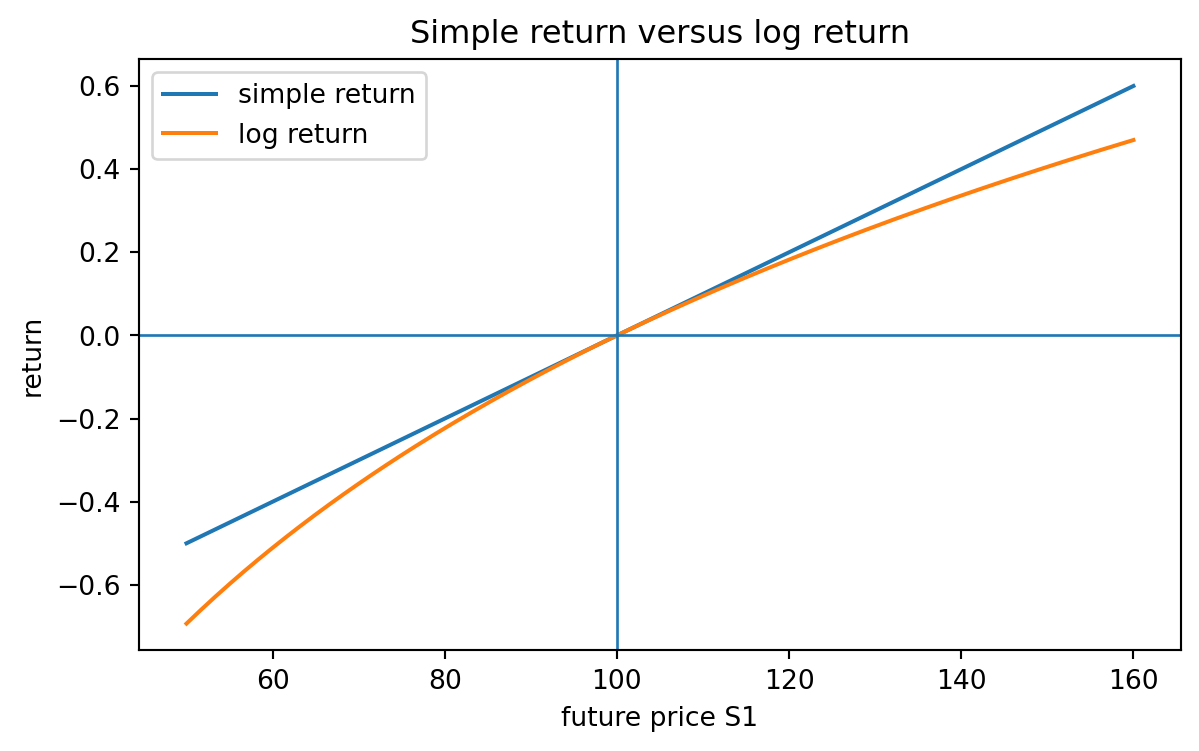
The following small example is intentionally simple. It helps students see how simple returns and log returns differ as price changes become larger.
import numpy as npimport pandas as pdimport matplotlib.pyplot as pltS0 =100S1 = np.linspace(50, 160, 200)simple_return = (S1 - S0) / S0log_return = np.log(S1 / S0)plt.figure(figsize=(7, 4))plt.plot(S1, simple_return, label="simple return")plt.plot(S1, log_return, label="log return")plt.axhline(0, linewidth=1)plt.axvline(S0, linewidth=1)plt.xlabel("future price S1")plt.ylabel("return")plt.title("Simple return versus log return")plt.legend()plt.show()
Simple return and log return as functions of the future price.
For small price changes, the two curves are close. For larger changes, the difference becomes visible.
Remark. For the interactive HTML version of this book, this chapter can later include a Plotly slider that changes \(S_0\) and shows the curves
A financial model is not just a collection of formulas. A mathematical model should specify:
the time set, such as \(\{0,1,\ldots,T\}\) or \([0,T]\);
the state space \(\Omega\);
the information available at each time;
the traded assets and their price processes;
the admissible trading strategies;
the rule for discounting;
the probability measure used for statistical modeling;
the pricing principle, usually no-arbitrage.
Without these components, formulas can be misleading. For example, the Black–Scholes formula is not just a formula for an option price; it is the result of assumptions about continuous trading, geometric Brownian motion, constant volatility, constant interest rate, no transaction costs, and replication.
The goal of this book is to make these assumptions visible.
4.16 1.15 Common Mistakes
Confusing payoff and price. A payoff occurs in the future and may be random. A price is known today.
Forgetting discounting. A dollar tomorrow is not the same as a dollar today when interest rates are nonzero.
Using physical probabilities for pricing. The expected payoff under \(\mathbb P\) is not generally the no-arbitrage price.
Ignoring admissible strategies. Arbitrage depends on what trading strategies are allowed.
Thinking no-arbitrage means no risk. No-arbitrage removes free profits; it does not remove uncertainty.
Treating models as reality. A model is useful when it clarifies structure and gives testable approximations.
4.17 1.16 Exercises
4.17.1 Conceptual exercises
Explain the difference between a price and a payoff.
Explain why discounting is necessary when comparing cash flows at different times.
Give an example of a situation where simple returns are more convenient than log returns.
Give an example of a situation where log returns are more convenient than simple returns.
Explain why an arbitrage opportunity is a mathematical inconsistency in a pricing model.
Explain the difference between \(\mathbb P\) and \(\mathbb Q\).
4.17.2 Computational exercises
Suppose \(S_0=50\) and \(S_1=55\). Compute the simple return and log return.
Suppose a stock moves from \(100\) to either \(130\) or \(90\), and the interest rate is \(4\%\). Compute the risk-neutral probability.
In the model from Exercise 8, price a European call option with strike \(K=100\) by replication.
Verify your answer to Exercise 9 using discounted risk-neutral expectation.
4.17.3 Linear algebra exercises
Consider a one-period model with three states and two risky assets. The payoff matrix is
In a one-period binomial model, derive the formula
\[
q=\frac{(1+r)-d}{u-d}.
\]
Show that the no-arbitrage condition for the binomial stock model is
\[
d<1+r<u.
\]
4.18 1.17 Chapter Summary
This chapter introduced mathematical finance as the study of uncertain cash flows, prices, portfolios, and information. The main ideas are:
prices today are different from future payoffs;
returns measure relative changes in price;
discounting converts future cash flows into present value;
portfolios create linear combinations of payoff vectors;
arbitrage is a free-lunch trading strategy and should be excluded from a pricing model;
one-period pricing can be understood through replication, state prices, and risk-neutral probabilities;
the physical probability measure \(\mathbb P\) describes statistical behavior, while the pricing measure \(\mathbb Q\) supports no-arbitrage valuation;
market completeness is a linear algebra condition.
The next chapter studies discounting, compounding, present value, future value, and bond prices in greater detail.
Source Code
---title: "Chapter 1. What Is Mathematical Finance?"---::: {.chapter-objectives}## Learning GoalsBy the end of this chapter, students should be able to:- describe mathematical finance as the study of prices, cash flows, portfolios, uncertainty, and information;- distinguish prices, payoffs, simple returns, log returns, and portfolio values;- explain why arbitrage is a mathematical inconsistency in a financial model;- represent one-period asset payoffs as vectors and portfolios as linear combinations;- connect no-arbitrage pricing with linear algebra, probability, and discounting;- explain the difference between the real-world probability measure and the pricing probability measure;- understand the role of models: useful approximations, not exact descriptions of markets.:::::: {.hero-box}Mathematical finance begins with a simple question: **what is a fair price today for a future uncertain cash flow?**The answer is not just a formula. It requires a model of uncertainty, a model of information, and a precise rule describing what trading strategies are allowed.:::## 1.1 Why Mathematical Finance?A financial asset has a price today and an uncertain value in the future. A derivative is a contract whose payoff depends on one or more underlying assets. A portfolio is a collection of positions in assets. Mathematical finance studies these objects using probability, linear algebra, optimization, stochastic processes, and numerical computation.The central mathematical problem is this:> Given a future payoff, determine its present value under assumptions that exclude arbitrage.For example, a European call option with strike $K$ and maturity $T$ pays$$(S_T-K)^+ = \max(S_T-K,0)$$at time $T$. Its value today depends on the possible future values of $S_T$, the interest rate, the market information, and whether the payoff can be replicated by trading other assets.This book develops the mathematical ideas behind such questions. We begin in discrete time, where the main ideas are transparent. Later chapters move to Brownian motion, stochastic calculus, Black--Scholes theory, interest-rate models, risk measures, and portfolio optimization.## 1.2 Prices, Payoffs, and ReturnsLet $S_t$ denote the price of an asset at time $t$. In a deterministic setting, $S_t$ is just a number. In a stochastic model, $S_t$ is a random variable because future prices are uncertain.### Simple returnThe **simple return** from time $t$ to time $t+1$ is$$R_{t+1}=\frac{S_{t+1}-S_t}{S_t}.$$Equivalently,$$S_{t+1}=S_t(1+R_{t+1}).$$The simple return measures relative gain or loss. If $S_t=100$ and $S_{t+1}=108$, then $R_{t+1}=0.08$.### Gross returnThe **gross return** is$$G_{t+1}=1+R_{t+1}=\frac{S_{t+1}}{S_t}.$$Gross returns multiply naturally over time:$$\frac{S_T}{S_0}=G_1G_2\cdots G_T.$$### Log returnThe **log return** is$$r_{t+1}=\log \frac{S_{t+1}}{S_t}.$$Log returns add naturally over time:$$\log\frac{S_T}{S_0}=r_1+r_2+\cdots+r_T.$$This additive property is one reason log returns are common in probability models and statistical estimation.::: {.definition}**Definition 1.1 (Price process).** A price process is a sequence of random variables$$S_0,S_1,\ldots,S_T,$$where $S_t$ represents the price of an asset at time $t$. The value $S_0$ is usually known at time $0$, while $S_1,\ldots,S_T$ may be random.:::::: {.remark}Simple returns are natural for portfolio accounting. Log returns are natural for probability modeling. They are close when returns are small because$$\log(1+x)\approx x$$for small $x$.:::## 1.3 Riskless Asset and DiscountingA riskless asset, often called a bank account or money-market account, grows at a known rate. In a one-period model with interest rate $r$, one dollar invested at time $0$ becomes $1+r$ dollars at time $1$.Let$$B_0=1, \qquad B_1=1+r.$$If a deterministic cash flow $X$ is received at time $1$, its present value is$$\frac{X}{1+r}.$$More generally, if a riskless bank account satisfies$$B_t=(1+r)^t,$$then the discounted value of a price process $S_t$ is$$\widetilde S_t=\frac{S_t}{B_t}.$$Discounting converts future dollars into time-$0$ dollars. Many pricing formulas are simplest when written in terms of discounted values.::: {.definition}**Definition 1.2 (Discounted price).** Given a riskless account $B_t>0$, the discounted price of an asset $S_t$ is$$\widetilde S_t=\frac{S_t}{B_t}.$$:::## 1.4 States of the World and Payoff VectorsIn a one-period model, uncertainty can be represented by a finite set of possible states:$$\Omega=\{\omega_1,\omega_2,\ldots,\omega_m\}.$$A payoff at time $1$ is a function$$X:\Omega\to \mathbb R.$$Since $\Omega$ has $m$ states, we may identify $X$ with a vector in $\mathbb R^m$:$$X=\begin{pmatrix}X(\omega_1)\\X(\omega_2)\\\vdots\\X(\omega_m)\end{pmatrix}.$$This is the first major connection between finance and linear algebra:> Future cash flows are vectors; portfolios form linear combinations of payoff vectors.Suppose there are $d$ traded assets. Let $S_0^j$ be the time-$0$ price of asset $j$, and let $S_1^j(\omega_i)$ be its time-$1$ payoff in state $\omega_i$. A portfolio is a vector$$\theta=(\theta_1,\ldots,\theta_d)^\top,$$where $\theta_j$ is the number of units held in asset $j$.The initial cost of the portfolio is$$V_0(\theta)=\sum_{j=1}^d \theta_jS_0^j.$$The future payoff is$$V_1(\theta,\omega_i)=\sum_{j=1}^d \theta_jS_1^j(\omega_i).$$In matrix form, let $A$ be the $m\times d$ payoff matrix whose $j$th column is the payoff vector of asset $j$:$$A=\begin{pmatrix}S_1^1(\omega_1) & \cdots & S_1^d(\omega_1)\\\vdots & \ddots & \vdots\\S_1^1(\omega_m) & \cdots & S_1^d(\omega_m)\end{pmatrix}.$$Then the payoff of portfolio $\theta$ is$$A\theta.$$## 1.5 Portfolios and Self-Financing TradingA portfolio describes holdings in assets. In a one-period model, a portfolio is chosen at time $0$ and produces a payoff at time $1$. In a multi-period model, the portfolio may be adjusted over time.A trading strategy is **self-financing** if all changes in the portfolio are paid for by selling and buying assets within the portfolio, with no external cash added or removed after the initial investment.In discrete time, if $\theta_t$ denotes the holdings during the period $(t,t+1]$, then the portfolio value is$$V_t=\theta_t\cdot S_t.$$The self-financing condition says that changes in wealth come only from price changes:$$V_{t+1}-V_t=\theta_t\cdot(S_{t+1}-S_t).$$This condition matters because pricing by replication only makes sense when the replicating strategy does not secretly inject extra money.::: {.definition}**Definition 1.3 (Self-financing strategy).** A trading strategy is self-financing if, after the initial portfolio is formed, all future changes in portfolio holdings are financed entirely by reallocating wealth among the traded assets.:::## 1.6 ArbitrageArbitrage is the mathematical expression of a free lunch. It is a trading strategy with no possible loss, no initial cost, and positive gain in at least one state.::: {.definition}**Definition 1.4 (Arbitrage in a one-period model).** A portfolio $\theta$ is an arbitrage if$$V_0(\theta)\le 0,$$$$V_1(\theta,\omega)\ge 0\quad \text{for all }\omega\in\Omega,$$and$$V_1(\theta,\omega)>0\quad \text{for at least one }\omega\in\Omega.$$:::A model with arbitrage is internally inconsistent for pricing. If a payoff can be obtained for two different prices, then buying the cheaper version and selling the more expensive version produces a riskless profit.No-arbitrage is not the statement that real markets never have mispricings. Rather, it is a modeling principle: in a liquid competitive market, large obvious arbitrages should not persist. Therefore a mathematical pricing model should not contain arbitrage opportunities as structural features.## 1.7 A First One-Period ModelConsider a one-period model with two possible states: up and down.At time $0$, a stock has price$$S_0=100.$$At time $1$, it can be$$S_1(u)=120,\qquad S_1(d)=80.$$The riskless asset grows from$$B_0=1$$to$$B_1=1.05.$$A European call option with strike $K=100$ has payoff$$C_1=(S_1-K)^+.$$Thus$$C_1(u)=20,\qquad C_1(d)=0.$$We ask: what should $C_0$ be?### ReplicationTry to replicate the option using $\Delta$ shares of stock and $b$ dollars in the bank account at time $0$. The time-$1$ value of this portfolio is$$\Delta S_1 + b(1.05).$$To replicate the call payoff, solve$$120\Delta+1.05b=20,$$$$80\Delta+1.05b=0.$$Subtracting the second equation from the first gives$$40\Delta=20,$$so$$\Delta=\frac12.$$Substituting into the second equation gives$$80\cdot \frac12+1.05b=0,$$so$$b=-\frac{40}{1.05}.$$Therefore the time-$0$ cost of the replicating portfolio is$$C_0=\Delta S_0+b=\frac12\cdot 100-\frac{40}{1.05}\approx 11.9048.$$The no-arbitrage price of the call is approximately $11.9048$.::: {.example}**Example 1.1 (Pricing by replication).** The option payoff $(20,0)$ can be written as a linear combination of the stock payoff $(120,80)$ and the bond payoff $(1.05,1.05)$:$$(20,0)=\frac12(120,80)-\frac{40}{1.05}(1.05,1.05).$$Thus the option price must equal the same linear combination of today's prices:$$C_0=\frac12(100)-\frac{40}{1.05}.$$:::## 1.8 Risk-Neutral ProbabilityThe same price can be written as a discounted expected payoff, but not necessarily under the real-world probability.Let $q$ be the probability of the up state under a new probability measure $\mathbb Q$. We choose $q$ so that the discounted stock price is a martingale:$$S_0=\frac{1}{1+r}\mathbb E^{\mathbb Q}[S_1].$$In this example,$$100=\frac{1}{1.05}\left(120q+80(1-q)\right).$$Therefore$$105=80+40q,$$so$$q=\frac{25}{40}=0.625.$$Then the option price is$$C_0=\frac{1}{1.05}\mathbb E^{\mathbb Q}[C_1]=\frac{1}{1.05}\left(0.625\cdot 20+0.375\cdot 0\right)\approx 11.9048.$$This agrees with replication.::: {.definition}**Definition 1.5 (Risk-neutral probability in a one-period binomial model).** The risk-neutral probability $q$ is the probability under which the discounted stock price has no drift:$$S_0=\frac{1}{1+r}\left(qS_1(u)+(1-q)S_1(d)\right).$$Equivalently, if $S_1(u)=uS_0$ and $S_1(d)=dS_0$, then$$q=\frac{(1+r)-d}{u-d}.$$:::::: {.remark}The risk-neutral probability is not introduced because investors are risk-neutral. It is introduced because no-arbitrage prices can often be written as discounted expectations under a special probability measure. This measure is a pricing tool.:::## 1.9 Physical Probability Versus Pricing ProbabilityThere are two different probability measures that students must keep separate.The **physical probability measure**, often denoted by $\mathbb P$, describes the statistical behavior of the market. It is used for estimation, forecasting, simulation, and risk management.The **risk-neutral probability measure**, often denoted by $\mathbb Q$, is used for pricing. Under $\mathbb Q$, discounted traded asset prices are martingales.In general,$$\mathbb P\ne \mathbb Q.$$A common beginner mistake is to price an option by taking the expected payoff under the real-world probability and then discounting. That is usually not correct. The correct no-arbitrage pricing formula uses the pricing measure:$$V_0=\frac{1}{1+r}\mathbb E^{\mathbb Q}[V_1],$$not generally$$V_0=\frac{1}{1+r}\mathbb E^{\mathbb P}[V_1].$$The real-world measure may assign a higher probability to the up state because investors expect the stock to grow. The pricing measure adjusts probabilities so that expected discounted gains of traded assets vanish.## 1.10 No-Arbitrage as Linear AlgebraIn a finite one-period model, no-arbitrage has a clean geometric interpretation.Let $p\in\mathbb R^d$ be the vector of time-$0$ asset prices, and let $A\in\mathbb R^{m\times d}$ be the matrix of time-$1$ payoffs. A portfolio $\theta\in\mathbb R^d$ has initial cost$$p\cdot \theta$$and payoff$$A\theta.$$An arbitrage exists if there is a vector $\theta$ such that$$p\cdot\theta\le 0,$$$$A\theta\ge 0,$$with strict positivity in at least one state.No-arbitrage means no such vector exists.This is a separation problem in finite-dimensional linear algebra. Roughly speaking, if no portfolio gives a free nonnegative payoff, then there exists a positive vector of state prices that assigns the correct present value to every traded payoff.::: {.theorem}**Theorem 1.1 (One-period no-arbitrage principle, informal finite-state version).** In a finite one-period market, absence of arbitrage is equivalent to the existence of strictly positive state prices that correctly price all traded assets.That is, there exists a vector $\pi=(\pi_1,\ldots,\pi_m)$ with $\pi_i>0$ such that$$S_0^j=\sum_{i=1}^m \pi_i S_1^j(\omega_i)$$for each traded asset $j$.:::The vector $\pi$ is called a **state-price vector**. It tells us the time-$0$ price of one dollar paid in a particular future state.If the riskless asset satisfies $B_0=1$ and $B_1=1+r$, then the state prices satisfy$$\sum_{i=1}^m \pi_i=\frac{1}{1+r}.$$Therefore one can define risk-neutral probabilities by$$q_i=(1+r)\pi_i.$$Then$$q_i>0,\qquad\sum_{i=1}^m q_i=1,$$and prices can be written as discounted expectations:$$S_0^j=\frac{1}{1+r}\sum_{i=1}^m q_iS_1^j(\omega_i).$$## 1.11 Complete and Incomplete MarketsA market is **complete** if every payoff can be replicated by trading the available assets. In linear algebra terms, this means that the columns of the payoff matrix span the whole payoff space.::: {.definition}**Definition 1.6 (Market completeness).** In a finite one-period model with $m$ states and payoff matrix $A\in\mathbb R^{m\times d}$, the market is complete if every payoff vector $X\in\mathbb R^m$ can be written as$$X=A\theta$$for some portfolio $\theta\in\mathbb R^d$.:::Thus the market is complete exactly when$$\operatorname{rank}(A)=m.$$If the market is complete, every payoff has a unique no-arbitrage price. If the market is incomplete, some payoffs cannot be replicated exactly. Then no-arbitrage may give a range of possible prices instead of one unique price.This distinction becomes important later for stochastic volatility, jump models, credit risk, and many realistic financial markets.## 1.12 A Small Python CheckThe following code verifies the binomial call option calculation from Section 1.7.```{python}#| label: ch01-binomial-call-check#| echo: trueS0 =100Su =120Sd =80r =0.05K =100Cu =max(Su - K, 0)Cd =max(Sd - K, 0)# Replication: solve Delta*Su + b*(1+r) = Cu,# Delta*Sd + b*(1+r) = Cd.Delta = (Cu - Cd) / (Su - Sd)b = (Cd - Delta * Sd) / (1+ r)C0_replication = Delta * S0 + b# Risk-neutral probabilityq = ((1+ r) * S0 - Sd) / (Su - Sd)C0_risk_neutral = (q * Cu + (1- q) * Cd) / (1+ r)print("Delta:", Delta)print("Bank account position:", b)print("Risk-neutral probability q:", q)print("Price by replication:", C0_replication)print("Price by risk-neutral expectation:", C0_risk_neutral)```The two prices agree because they are two descriptions of the same no-arbitrage principle.## 1.13 Interactive Visualization: Returns and Log ReturnsThe following small example is intentionally simple. It helps students see how simple returns and log returns differ as price changes become larger.```{python}#| label: ch01-return-comparison#| echo: true#| fig-cap: "Simple return and log return as functions of the future price."import numpy as npimport pandas as pdimport matplotlib.pyplot as pltS0 =100S1 = np.linspace(50, 160, 200)simple_return = (S1 - S0) / S0log_return = np.log(S1 / S0)plt.figure(figsize=(7, 4))plt.plot(S1, simple_return, label="simple return")plt.plot(S1, log_return, label="log return")plt.axhline(0, linewidth=1)plt.axvline(S0, linewidth=1)plt.xlabel("future price S1")plt.ylabel("return")plt.title("Simple return versus log return")plt.legend()plt.show()```For small price changes, the two curves are close. For larger changes, the difference becomes visible.::: {.remark}For the interactive HTML version of this book, this chapter can later include a Plotly slider that changes $S_0$ and shows the curves$$R=\frac{S_1-S_0}{S_0}\qquad \text{and} \qquadr=\log\frac{S_1}{S_0}.$$:::## 1.14 What Makes a Model Mathematical?A financial model is not just a collection of formulas. A mathematical model should specify:1. the time set, such as $\{0,1,\ldots,T\}$ or $[0,T]$;2. the state space $\Omega$;3. the information available at each time;4. the traded assets and their price processes;5. the admissible trading strategies;6. the rule for discounting;7. the probability measure used for statistical modeling;8. the pricing principle, usually no-arbitrage.Without these components, formulas can be misleading. For example, the Black--Scholes formula is not just a formula for an option price; it is the result of assumptions about continuous trading, geometric Brownian motion, constant volatility, constant interest rate, no transaction costs, and replication.The goal of this book is to make these assumptions visible.## 1.15 Common Mistakes1. **Confusing payoff and price.** A payoff occurs in the future and may be random. A price is known today.2. **Forgetting discounting.** A dollar tomorrow is not the same as a dollar today when interest rates are nonzero.3. **Using physical probabilities for pricing.** The expected payoff under $\mathbb P$ is not generally the no-arbitrage price.4. **Ignoring admissible strategies.** Arbitrage depends on what trading strategies are allowed.5. **Thinking no-arbitrage means no risk.** No-arbitrage removes free profits; it does not remove uncertainty.6. **Treating models as reality.** A model is useful when it clarifies structure and gives testable approximations.## 1.16 Exercises### Conceptual exercises1. Explain the difference between a price and a payoff.2. Explain why discounting is necessary when comparing cash flows at different times.3. Give an example of a situation where simple returns are more convenient than log returns.4. Give an example of a situation where log returns are more convenient than simple returns.5. Explain why an arbitrage opportunity is a mathematical inconsistency in a pricing model.6. Explain the difference between $\mathbb P$ and $\mathbb Q$.### Computational exercises7. Suppose $S_0=50$ and $S_1=55$. Compute the simple return and log return.8. Suppose a stock moves from $100$ to either $130$ or $90$, and the interest rate is $4\%$. Compute the risk-neutral probability.9. In the model from Exercise 8, price a European call option with strike $K=100$ by replication.10. Verify your answer to Exercise 9 using discounted risk-neutral expectation.### Linear algebra exercises11. Consider a one-period model with three states and two risky assets. The payoff matrix is$$A=\begin{pmatrix}2 & 1\\1 & 1\\0 & 1\end{pmatrix}.$$Determine whether the payoff $X=(1,1,1)^\top$ can be replicated.12. In the same model, determine whether the payoff $Y=(1,0,1)^\top$ can be replicated.13. Explain the relationship between market completeness and the rank of the payoff matrix.14. Suppose a payoff matrix has rank less than the number of states. What does this imply about completeness?### Proof-based exercises15. Prove that gross returns multiply over time:$$\frac{S_T}{S_0}=\prod_{t=1}^T \frac{S_t}{S_{t-1}}.$$16. Prove that log returns add over time:$$\log\frac{S_T}{S_0}=\sum_{t=1}^T \log\frac{S_t}{S_{t-1}}.$$17. In a one-period binomial model, derive the formula$$q=\frac{(1+r)-d}{u-d}.$$18. Show that the no-arbitrage condition for the binomial stock model is$$d<1+r<u.$$## 1.17 Chapter SummaryThis chapter introduced mathematical finance as the study of uncertain cash flows, prices, portfolios, and information. The main ideas are:- prices today are different from future payoffs;- returns measure relative changes in price;- discounting converts future cash flows into present value;- portfolios create linear combinations of payoff vectors;- arbitrage is a free-lunch trading strategy and should be excluded from a pricing model;- one-period pricing can be understood through replication, state prices, and risk-neutral probabilities;- the physical probability measure $\mathbb P$ describes statistical behavior, while the pricing measure $\mathbb Q$ supports no-arbitrage valuation;- market completeness is a linear algebra condition.The next chapter studies discounting, compounding, present value, future value, and bond prices in greater detail.