27  Chapter 24. Stochastic Volatility Models

27.1 Learning Goals

By the end of this chapter, students should be able to:

• explain why constant-volatility Black–Scholes models do not reproduce volatility clustering and volatility smiles;
• distinguish historical volatility, instantaneous variance, implied volatility, and realized variance;
• write a two-factor stochastic volatility model under the physical measure \(\mathbb P\) and under the risk-neutral measure \(\mathbb Q\);
• derive the log-price dynamics in a stochastic volatility model using Itô’s formula;
• explain how correlation between price shocks and volatility shocks creates skew;
• formulate the Heston model and interpret each parameter;
• state the Feller condition for the CIR variance process and explain what it means;
• derive the pricing PDE for a European option in a stochastic volatility model;
• explain why stochastic volatility models are typically incomplete;
• simulate Heston paths and use Monte Carlo to estimate option prices and implied volatility curves;
• use AI tools to audit stochastic volatility notation, simulation code, and calibration interpretation.

The Black–Scholes model assumes a constant volatility \(\sigma\). This assumption gives a beautiful closed-form formula, but it also predicts a flat implied-volatility surface. Real option markets usually show smiles, skews, and term structures.

Stochastic volatility models replace the constant parameter \(\sigma^2\) by a random variance process \(v_t\):

\[ \frac{dS_t}{S_t}=\mu_t\,dt+\sqrt{v_t}\,dW_t^S. \]

The main mathematical idea is simple but powerful: the stock price is random, and the volatility of the stock price is also random. The result is a two-factor model that can capture volatility clustering, leverage effects, and implied-volatility smiles more realistically than constant-volatility Black–Scholes.

27.2 24.1 Why Stochastic Volatility?

In the Black–Scholes model under the physical measure,

\[ dS_t=\mu S_t\,dt+\sigma S_t\,dW_t, \]

volatility is a constant parameter. Consequently, over a short interval of length \(\Delta t\),

\[ \operatorname{Var}\left(\frac{\Delta S_t}{S_t}\mid \mathcal F_t\right) \approx \sigma^2\Delta t. \]

This is mathematically clean, but financial return data often show features inconsistent with constant volatility.

27.2.1 Empirical motivation

Common empirical observations include:

1. Volatility clustering: large price moves tend to be followed by large price moves, and quiet periods tend to be followed by quiet periods.
2. Leverage effect: negative equity returns are often associated with increases in future volatility.
3. Heavy tails: return distributions have more extreme observations than a normal model with constant variance.
4. Implied-volatility smile or skew: Black–Scholes implied volatility depends on strike and maturity, even though the model assumes one constant \(\sigma\).

A stochastic volatility model is designed to give the volatility its own dynamics. Instead of assuming that volatility is fixed, we model the conditional variance as an evolving random state variable.

27.3 Instantaneous variance

In a diffusion model

\[ \frac{dS_t}{S_t}=\mu_t\,dt+\sqrt{v_t}\,dW_t^S, \]

the process \(v_t\) is called the instantaneous variance process. The instantaneous volatility is \(\sqrt{v_t}\).

The conditional variance over a small time step is approximately

\[ \operatorname{Var}\left(\frac{dS_t}{S_t}\mid\mathcal F_t\right)=v_t\,dt. \]

Thus, \(v_t\) plays the same local role as \(\sigma^2\) in Black–Scholes, but it is now random and time-varying.

27.4 24.2 Four Notions of Volatility

Students often confuse several different notions of volatility. A clean mathematical finance treatment should separate them.

Name	Symbol	Meaning	Source
Instantaneous variance	\(v_t\)	local conditional variance rate	model state
Instantaneous volatility	\(\sqrt{v_t}\)	local conditional standard deviation rate	model state
Realized variance	\(\sum_i (\Delta \log S_i)^2\)	observed path variation	historical data
Implied volatility	\(\sigma_{\mathrm{imp}}(K,T)\)	Black–Scholes volatility matching a market option price	option market

Realized variance over \([0,T]\) is a discrete approximation to quadratic variation:

\[ \operatorname{RV}_{0,T} = \sum_{i=1}^n \left(\log S_{t_i}-\log S_{t_{i-1}}\right)^2 \approx \int_0^T v_t\,dt. \]

Implied volatility is different. If \(C^{\mathrm{mkt}}(K,T)\) is a market call price, then the implied volatility is the value \(\sigma_{\mathrm{imp}}\) satisfying

\[ C^{\mathrm{BS}}(S_0,K,r,T,\sigma_{\mathrm{imp}})=C^{\mathrm{mkt}}(K,T). \]

If the Black–Scholes model were exactly correct with constant volatility \(\sigma\), then \(\sigma_{\mathrm{imp}}(K,T)\) would be constant in \(K\) and \(T\). A non-flat implied-volatility surface is one of the main motivations for richer models.

27.5 24.3 General Two-Factor Stochastic Volatility Model

A common stochastic volatility model has two Brownian motions:

\[ \frac{dS_t}{S_t}=\mu(t,S_t,v_t)\,dt+\sqrt{v_t}\,dW_t^S, \]

\[ dv_t=a(t,v_t)\,dt+b(t,v_t)\,dW_t^v, \]

with instantaneous correlation

\[ d\langle W^S,W^v\rangle_t=\rho\,dt, \qquad -1\le \rho\le 1. \]

Equivalently, one may write

\[ dW_t^v=\rho\,dW_t^S+\sqrt{1-\rho^2}\,dW_t^\perp, \]

where \(W^\perp\) is a Brownian motion independent of \(W^S\).

Remark (The role of correlation). The parameter \(\rho\) controls the instantaneous relationship between price shocks and variance shocks. In equity markets, \(\rho\) is often negative in calibrated models. Negative \(\rho\) means that downward price shocks tend to arrive with upward volatility shocks.

The quadratic variations and covariation are

\[ d\langle \log S\rangle_t=v_t\,dt, \]

\[ d\langle v\rangle_t=b(t,v_t)^2\,dt, \]

and

\[ d\langle \log S,v\rangle_t=\rho\sqrt{v_t}\,b(t,v_t)\,dt. \]

These covariation formulas are central when deriving option-pricing PDEs.

27.6 24.4 Physical Measure and Risk-Neutral Measure

Under the physical probability measure \(\mathbb P\), the stock drift describes real-world expected return:

\[ \frac{dS_t}{S_t}=\mu_t\,dt+\sqrt{v_t}\,dW_t^{S,\mathbb P}. \]

For option pricing, we usually work under a risk-neutral measure \(\mathbb Q\):

\[ \frac{dS_t}{S_t}=r_t\,dt+\sqrt{v_t}\,dW_t^{S,\mathbb Q}. \]

The variance process also changes drift when we change measure. A typical notation is

\[ dv_t=a^{\mathbb P}(t,v_t)\,dt+b(t,v_t)\,dW_t^{v,\mathbb P} \]

under \(\mathbb P\) and

\[ dv_t=a^{\mathbb Q}(t,v_t)\,dt+b(t,v_t)\,dW_t^{v,\mathbb Q} \]

under \(\mathbb Q\).

The difference between \(a^{\mathbb P}\) and \(a^{\mathbb Q}\) is related to the market price of volatility risk.

27.7 Common mistake

Do not estimate a stochastic volatility model under \(\mathbb P\) from historical returns and then use the same drift parameters for option pricing without thinking about the change of measure. Historical estimation and risk-neutral calibration answer different questions.

For pricing European derivatives, we will usually write the model directly under \(\mathbb Q\).

27.8 24.5 The Heston Model

The most famous stochastic volatility model in mathematical finance is the Heston model. Under the risk-neutral measure \(\mathbb Q\), it is usually written as

\[ \frac{dS_t}{S_t}=r\,dt+\sqrt{v_t}\,dW_t^S, \]

\[ dv_t=\kappa(\theta-v_t)\,dt+\xi\sqrt{v_t}\,dW_t^v, \]

with

\[ d\langle W^S,W^v\rangle_t=\rho\,dt. \]

Here:

Parameter	Interpretation
\(r\)	risk-free rate
\(v_t\)	instantaneous variance
\(\kappa\)	mean-reversion speed of variance
\(\theta\)	long-run mean variance
\(\xi\)	volatility of variance, often called vol-of-vol
\(\rho\)	correlation between return and variance shocks

The variance process is a Cox–Ingersoll–Ross type square-root process. It mean-reverts toward \(\theta\) and has diffusion coefficient \(\xi\sqrt{v_t}\).

27.9 Heston model

The Heston model under \(\mathbb Q\) is

\[ \begin{aligned} \frac{dS_t}{S_t}&=r\,dt+\sqrt{v_t}\,dW_t^S,\\ dv_t&=\kappa(\theta-v_t)\,dt+\xi\sqrt{v_t}\,dW_t^v,\\ d\langle W^S,W^v\rangle_t&=\rho\,dt. \end{aligned} \]

27.10 24.6 Mean Reversion of Variance

Ignoring the diffusion term for a moment, the deterministic part of the variance equation is

\[ \frac{dv_t}{dt}=\kappa(\theta-v_t). \]

Solving this ordinary differential equation gives

\[ v_t=\theta+(v_0-\theta)e^{-\kappa t}. \]

Thus:

• if \(v_0>\theta\), the drift is negative and pulls \(v_t\) downward;
• if \(v_0<\theta\), the drift is positive and pulls \(v_t\) upward;
• larger \(\kappa\) means faster mean reversion.

For the full CIR variance process,

\[ \mathbb E^{\mathbb Q}[v_t\mid v_0] = \theta+(v_0-\theta)e^{-\kappa t}. \]

The conditional expectation has the same form as the deterministic mean-reversion solution.

27.11 24.7 Positivity and the Feller Condition

Because \(v_t\) represents variance, it should remain nonnegative. The square-root diffusion coefficient \(\xi\sqrt{v_t}\) helps preserve nonnegativity.

For the CIR variance process

\[ dv_t=\kappa(\theta-v_t)\,dt+\xi\sqrt{v_t}\,dW_t, \]

the boundary behavior at zero is controlled by the Feller condition:

\[ 2\kappa\theta\ge \xi^2. \]

If this condition holds, the process stays strictly positive when \(v_0>0\). If it fails, the process may touch zero, but it remains nonnegative in the continuous-time model.

Remark (Numerical versus theoretical positivity). The continuous-time CIR process is nonnegative. A naive Euler discretization, however, can produce negative variance values. This is a numerical artifact, not a feature of the model.

Common simulation fixes include:

• full truncation Euler;
• reflection schemes;
• exact simulation of the CIR process;
• quadratic-exponential schemes.

For an introductory mathematical finance course, full truncation Euler is easy to implement and useful pedagogically.

27.12 24.8 Log-Price Dynamics

Let

\[ X_t=\log S_t. \]

Using Itô’s formula with

\[ dS_t=rS_t\,dt+\sqrt{v_t}S_t\,dW_t^S, \]

we obtain

\[ dX_t= \left(r-\frac12 v_t\right)dt+\sqrt{v_t}\,dW_t^S. \]

Therefore,

\[ X_T = X_0+rT-\frac12\int_0^T v_t\,dt + \int_0^T\sqrt{v_t}\,dW_t^S. \]

This formula reveals the key difference from Black–Scholes. In Black–Scholes, \(v_t=\sigma^2\) is constant, so \(X_T\) is normally distributed. In Heston, the integrated variance

\[ \int_0^T v_t\,dt \]

is random, so the log-price distribution becomes a mixture-like distribution with heavier tails and skew.

27.13 24.9 Conditional Normality Given the Variance Path

Suppose temporarily that the variance path \((v_t)_{0\le t\le T}\) is known. If \(\rho=0\), the Brownian motion driving returns is independent of the Brownian motion driving variance. Conditional on the variance path,

\[ \log S_T \mid (v_t)_{0\le t\le T} \sim N\left( \log S_0+rT-\frac12\int_0^T v_t\,dt, \int_0^T v_t\,dt \right). \]

This is an important intuition: stochastic volatility creates a random variance mixture of normal distributions. Random variance mixtures often have heavier tails than a single normal distribution.

When \(\rho\ne 0\), the conditioning is more subtle because stock and variance shocks are correlated, but the same intuition remains useful: randomness in variance changes the shape of the return distribution.

27.14 24.10 Interactive Example: Heston Sample Paths

The following interactive demo simulates sample paths from a simple full-truncation Euler approximation. Increase vol-of-vol \(\xi\) to make variance more random. Change \(\rho\) to see how price and variance shocks are coupled.

27.14.1 Heston paths under risk-neutral dynamics

Vol-of-vol \(\xi\) 0.45

Correlation \(\rho\) -0.60

27.15 24.11 Pricing PDE for Stochastic Volatility Models

Let \(V(t,S_t,v_t)\) be the price of a European payoff \(H(S_T)\). Under a risk-neutral stochastic volatility model

\[ dS_t=rS_t\,dt+\sqrt{v_t}S_t\,dW_t^S, \]

\[ dv_t=a(t,v_t)\,dt+b(t,v_t)\,dW_t^v, \]

with

\[ d\langle W^S,W^v\rangle_t=\rho\,dt, \]

we apply the two-dimensional Itô formula to \(V(t,S,v)\). The second-order terms are

\[ (dS_t)^2=v_tS_t^2\,dt, \]

\[ (dv_t)^2=b(t,v_t)^2\,dt, \]

and

\[ dS_t\,dv_t=\rho S_t\sqrt{v_t}\,b(t,v_t)\,dt. \]

The infinitesimal generator under \(\mathbb Q\) is

\[ \mathcal L V = rS V_S+a(t,v)V_v +\frac12 vS^2V_{SS} +\rho S\sqrt v\,b(t,v)V_{Sv} +\frac12 b(t,v)^2V_{vv}. \]

The risk-neutral pricing PDE is

\[ V_t+\mathcal L V-rV=0, \]

with terminal condition

\[ V(T,S,v)=H(S). \]

For the Heston model, \(a(v)=\kappa(\theta-v)\) and \(b(v)=\xi\sqrt v\). Therefore,

\[ \boxed{ V_t+rS V_S+\kappa(\theta-v)V_v +\frac12 vS^2V_{SS} +\rho\xi vS V_{Sv} +\frac12\xi^2v V_{vv} -rV=0. } \]

Remark (Why the mixed derivative appears). The term \(\rho\xi vS V_{Sv}\) comes from the covariance between the stock-price shock and the variance shock. It disappears only when \(\rho=0\).

27.16 24.12 Incompleteness and Volatility Risk

In Black–Scholes, one Brownian motion drives one risky asset. The stock and bond are enough to replicate European claims. In a stochastic volatility model, there are usually two Brownian sources of risk:

\[ W^S \quad \text{and} \quad W^v. \]

But if the only traded risky asset is the stock \(S\), then there is only one directly traded source of randomness. The volatility shock cannot generally be hedged using the stock and bond alone.

27.17 Market incompleteness

A market is complete if every sufficiently regular contingent claim can be replicated by a self-financing trading strategy in traded assets. Stochastic volatility models are typically incomplete unless enough volatility-linked instruments are also traded.

In an incomplete market, no-arbitrage alone may not identify a unique risk-neutral measure. A modeler must specify a volatility risk premium, calibrate to option prices, or introduce additional traded instruments such as options or variance swaps.

This is a major conceptual difference from the Black–Scholes model. Stochastic volatility gives more realism but requires more modeling choices.

27.18 24.13 Heston Characteristic Function: Main Idea

One reason the Heston model is popular is that it has an affine structure. Although the density of \(S_T\) is not elementary, the characteristic function of \(\log S_T\) has a semi-closed form. Option prices can then be computed by Fourier inversion.

The affine form is

\[ \mathbb E^{\mathbb Q}\left[e^{iu\log S_T}\mid S_t=s,v_t=v\right] = \exp\left(A(\tau,u)+B(\tau,u)v+iu\log s\right), \]

where \(\tau=T-t\) and \(A,B\) solve Riccati-type ordinary differential equations.

For this book, the important lesson is not to memorize the full formula. The important mathematical ideas are:

1. the Heston model is a two-dimensional Markov diffusion;
2. its variance process is affine;
3. exponential-affine transforms reduce pricing integrals to ODEs;
4. Fourier methods convert characteristic functions into option prices.

This is a bridge between stochastic calculus, differential equations, and numerical finance.

27.19 24.14 Implied Volatility Smile and Skew

The Black–Scholes implied volatility of a model-generated price is defined by solving

\[ C^{\mathrm{BS}}(S_0,K,r,T,\sigma_{\mathrm{imp}})=C^{\mathrm{model}}(K,T). \]

In stochastic volatility models, \(\sigma_{\mathrm{imp}}(K,T)\) often varies with \(K\) and \(T\).

A negative correlation \(\rho\) tends to produce an equity-like skew. Intuitively, when the stock falls, variance tends to rise. This increases the value of downside-protection options and raises implied volatilities for low strikes.

27.19.1 Toy implied-volatility skew from stochastic volatility intuition

This demo is not a Heston pricing engine. It visualizes the qualitative relationship between vol-of-vol, correlation, and an implied-volatility curve.

Correlation \(\rho\) -0.60

Vol-of-vol \(\xi\) 0.45

27.20 24.15 Local Volatility versus Stochastic Volatility

A local volatility model has the form

\[ \frac{dS_t}{S_t}=r\,dt+\sigma_{\mathrm{loc}}(t,S_t)\,dW_t. \]

The volatility is random because it depends on \(S_t\), but it is not an additional random factor. Once \(t\) and \(S_t\) are known, the volatility is known.

A stochastic volatility model has the form

\[ \frac{dS_t}{S_t}=r\,dt+\sqrt{v_t}\,dW_t^S, \]

where \(v_t\) is its own stochastic process.

Model type	Volatility source	Markov state	Typical use
Black–Scholes	constant \(\sigma\)	\(S_t\)	closed-form benchmark
Local volatility	function \(\sigma_{\mathrm{loc}}(t,S_t)\)	\(S_t\)	exact fit to vanilla surface under idealized assumptions
Stochastic volatility	random factor \(v_t\)	\((S_t,v_t)\)	smiles, skews, volatility dynamics

Stochastic volatility models are often more natural for dynamics because they allow volatility to move independently of the current stock price.

27.21 24.16 Python Example: Simulating Heston Paths

import numpy as np
import pandas as pd
import matplotlib.pyplot as plt
from math import exp, log, sqrt, erf

rng = np.random.default_rng(7243)

S0 = 100.0
r = 0.03
T = 1.0
steps = 252
paths = 5000
v0 = 0.04
kappa = 2.0
theta = 0.04
xi = 0.45
rho = -0.60

def simulate_heston_full_truncation(
    S0=100.0, v0=0.04, r=0.03, kappa=2.0, theta=0.04,
    xi=0.45, rho=-0.60, T=1.0, steps=252, paths=5000, seed=7243
):
    """Full-truncation Euler simulation of the risk-neutral Heston model."""
    rng = np.random.default_rng(seed)
    dt = T / steps
    S = np.empty((paths, steps + 1))
    v = np.empty((paths, steps + 1))
    S[:, 0] = S0
    v[:, 0] = v0

    for n in range(steps):
        z1 = rng.standard_normal(paths)
        z2 = rng.standard_normal(paths)
        z_v = rho * z1 + np.sqrt(1 - rho**2) * z2
        v_plus = np.maximum(v[:, n], 0.0)

        S[:, n + 1] = S[:, n] * np.exp(
            (r - 0.5 * v_plus) * dt + np.sqrt(v_plus * dt) * z1
        )
        v[:, n + 1] = v[:, n] + kappa * (theta - v_plus) * dt + xi * np.sqrt(v_plus * dt) * z_v
        v[:, n + 1] = np.maximum(v[:, n + 1], 0.0)

    time_grid = np.linspace(0, T, steps + 1)
    return time_grid, S, v

time_grid, S_paths, v_paths = simulate_heston_full_truncation(paths=paths)
S_paths.shape, v_paths.shape

((5000, 253), (5000, 253))

The function returns both the stock-price paths and the variance paths. We keep \(v_t\) nonnegative by full truncation.

27.22 24.17 Python Example: Visualizing Price and Volatility Paths

plt.figure(figsize=(8, 4))
for i in range(8):
    plt.plot(time_grid, S_paths[i], alpha=0.85)
plt.xlabel("time")
plt.ylabel("stock price")
plt.title("Sample Heston stock-price paths")
plt.show()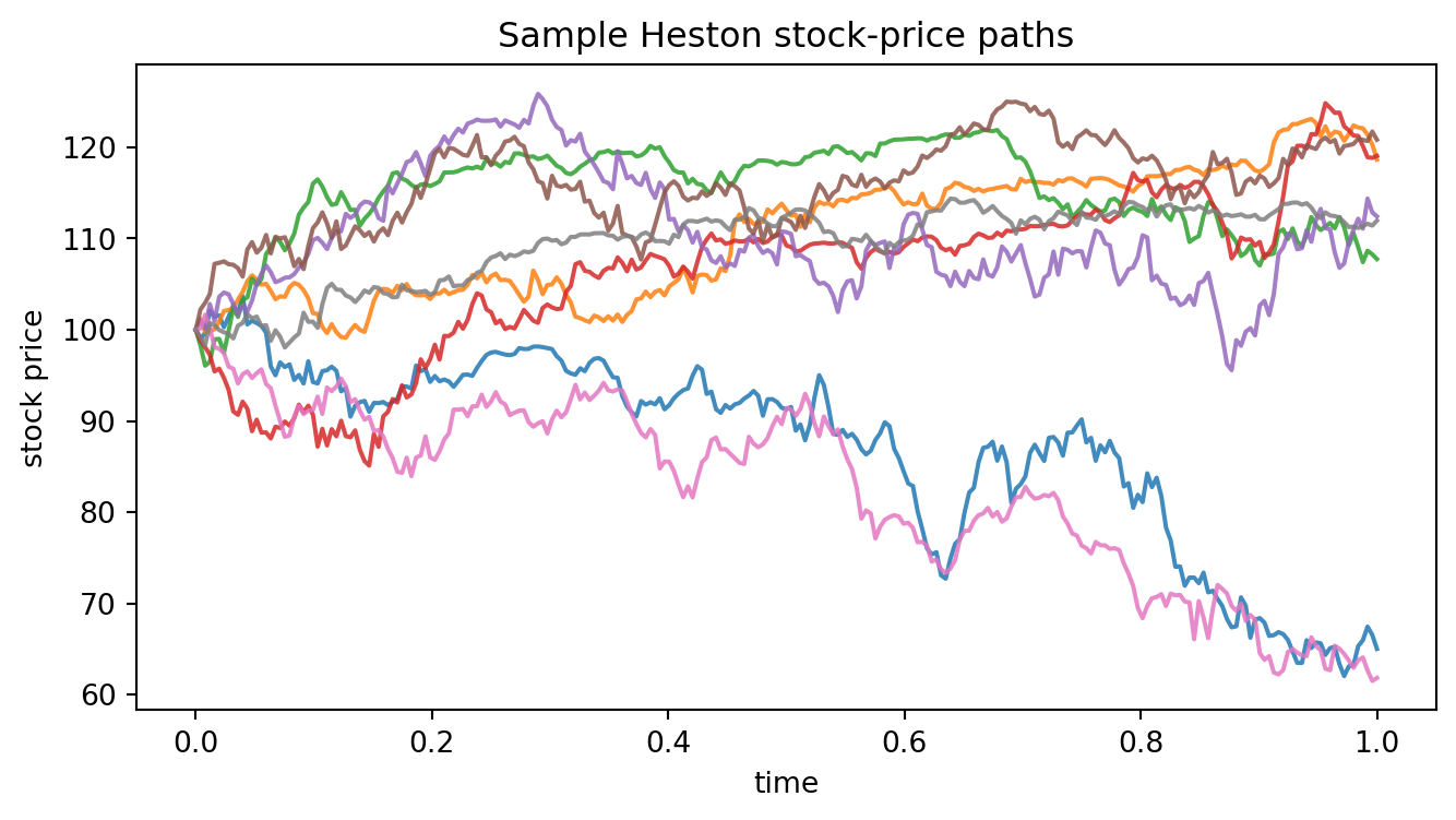

plt.figure(figsize=(8, 4))
for i in range(8):
    plt.plot(time_grid, np.sqrt(v_paths[i]), alpha=0.85)
plt.xlabel("time")
plt.ylabel("instantaneous volatility")
plt.title("Sample Heston volatility paths")
plt.show()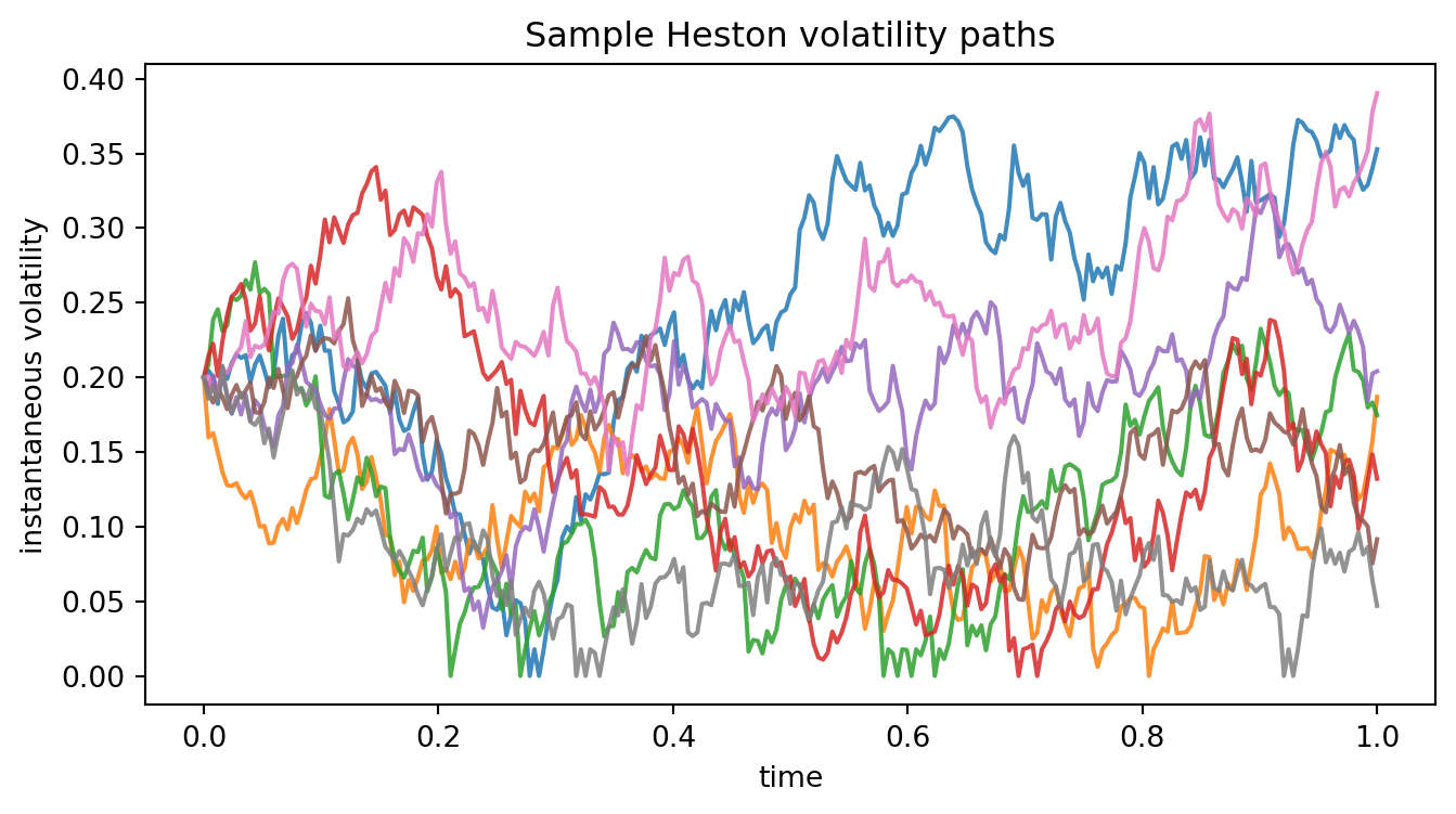

Students should compare these plots with geometric Brownian motion. In GBM, the volatility level is fixed. In Heston, calm and turbulent periods can occur within the same model.

27.23 24.18 Python Example: Mean Reversion and the Feller Condition

def feller_gap(kappa, theta, xi):
    return 2 * kappa * theta - xi**2

parameter_sets = pd.DataFrame({
    "kappa": [1.0, 2.0, 4.0],
    "theta": [0.04, 0.04, 0.04],
    "xi": [0.30, 0.45, 0.80]
})
parameter_sets["2 kappa theta - xi^2"] = [
    feller_gap(row.kappa, row.theta, row.xi)
    for row in parameter_sets.itertuples(index=False)
]
parameter_sets["Feller condition holds"] = parameter_sets["2 kappa theta - xi^2"] >= 0
parameter_sets

	kappa	theta	xi	2 kappa theta - xi^2	Feller condition holds
0	1.0	0.04	0.30	-0.0100	False
1	2.0	0.04	0.45	-0.0425	False
2	4.0	0.04	0.80	-0.3200	False

The Feller condition is sufficient for strict positivity, but it is not always imposed in market calibration. Calibrated Heston parameters sometimes violate it, especially when the market smile is steep.

27.24 24.19 Python Example: Realized Variance from Simulated Paths

For a simulated log-price path, realized variance is

\[ \sum_{i=1}^n (X_{t_i}-X_{t_{i-1}})^2. \]

The model integrated variance is approximately

\[ \int_0^T v_t\,dt. \]

log_returns = np.diff(np.log(S_paths), axis=1)
realized_variance = np.sum(log_returns**2, axis=1)
# NumPy compatibility: np.trapezoid was introduced in newer NumPy versions.
# np.trapz works in older environments, including many default conda setups.
integrated_variance = np.trapz(v_paths, x=time_grid, axis=1)

summary = pd.DataFrame({
    "quantity": ["realized variance", "integrated variance"],
    "sample mean": [realized_variance.mean(), integrated_variance.mean()],
    "sample std": [realized_variance.std(ddof=1), integrated_variance.std(ddof=1)]
})
summary

	quantity	sample mean	sample std
0	realized variance	0.039662	0.027500
1	integrated variance	0.039576	0.026977

In a fine time discretization, realized variance is a noisy pathwise approximation to integrated variance.

27.25 24.20 Python Example: Leverage Effect in Simulated Data

A negative \(\rho\) means that return shocks and variance shocks tend to move in opposite directions. We can observe this in simulated increments.

returns = np.diff(np.log(S_paths), axis=1).reshape(-1)
vol_changes = np.diff(v_paths, axis=1).reshape(-1)
np.corrcoef(returns, vol_changes)[0, 1]

-0.6006863638014469

The empirical correlation should be negative when \(\rho<0\), although discretization and drift terms make it different from exactly \(\rho\).

27.26 24.21 Python Example: Monte Carlo Option Prices

def heston_call_price_mc(K, S0=100.0, v0=0.04, r=0.03, kappa=2.0, theta=0.04,
                         xi=0.45, rho=-0.60, T=1.0, steps=252,
                         paths=30_000, seed=11):
    _, S, _ = simulate_heston_full_truncation(
        S0=S0, v0=v0, r=r, kappa=kappa, theta=theta,
        xi=xi, rho=rho, T=T, steps=steps, paths=paths, seed=seed
    )
    payoff = np.maximum(S[:, -1] - K, 0.0)
    price = np.exp(-r * T) * payoff.mean()
    se = np.exp(-r * T) * payoff.std(ddof=1) / np.sqrt(paths)
    return price, se

strikes = np.array([80, 90, 100, 110, 120])
prices = []
errors = []
for K in strikes:
    price, se = heston_call_price_mc(K, paths=12_000, seed=100 + int(K))
    prices.append(price)
    errors.append(se)

pd.DataFrame({"K": strikes, "Heston MC price": prices, "standard error": errors})

	K	Heston MC price	standard error
0	80	23.706447	0.148305
1	90	15.611880	0.128209
2	100	9.007966	0.102168
3	110	4.179888	0.071305
4	120	1.624125	0.045056

Monte Carlo estimates should always be reported with uncertainty. The standard error decreases like \(N^{-1/2}\).

27.27 24.22 Python Example: Implied Volatility from Heston Prices

def norm_cdf(x):
    return 0.5 * (1.0 + erf(x / sqrt(2.0)))

def bs_call_price(S0, K, r, T, sigma):
    if sigma <= 0 or T <= 0:
        return max(S0 - K * exp(-r * T), 0.0)
    d1 = (log(S0 / K) + (r + 0.5 * sigma**2) * T) / (sigma * sqrt(T))
    d2 = d1 - sigma * sqrt(T)
    return S0 * norm_cdf(d1) - K * exp(-r * T) * norm_cdf(d2)

def implied_vol_call(price, S0, K, r, T, low=1e-4, high=3.0, tol=1e-6, max_iter=100):
    intrinsic = max(S0 - K * exp(-r * T), 0.0)
    upper = S0
    if price < intrinsic - 1e-8 or price > upper + 1e-8:
        return np.nan
    lo, hi = low, high
    for _ in range(max_iter):
        mid = 0.5 * (lo + hi)
        val = bs_call_price(S0, K, r, T, mid)
        if val > price:
            hi = mid
        else:
            lo = mid
        if hi - lo < tol:
            break
    return 0.5 * (lo + hi)

implied_vols = [implied_vol_call(p, S0, K, r, T) for p, K in zip(prices, strikes)]
pd.DataFrame({"K": strikes, "Heston price": prices, "implied volatility": implied_vols})

	K	Heston price	implied volatility
0	80	23.706447	0.227847
1	90	15.611880	0.206149
2	100	9.007966	0.189511
3	110	4.179888	0.171124
4	120	1.624125	0.161910

A non-flat implied-volatility pattern indicates that the stochastic volatility model is producing option prices that cannot be represented by a single Black–Scholes volatility.

27.28 24.23 Python Example: Smile Plot from Monte Carlo Prices

plt.figure(figsize=(7, 4))
plt.plot(strikes, implied_vols, marker="o")
plt.axhline(np.sqrt(theta), linestyle="--", label="sqrt(theta)")
plt.xlabel("strike")
plt.ylabel("Black-Scholes implied volatility")
plt.title("Implied volatilities from simulated Heston option prices")
plt.legend()
plt.show()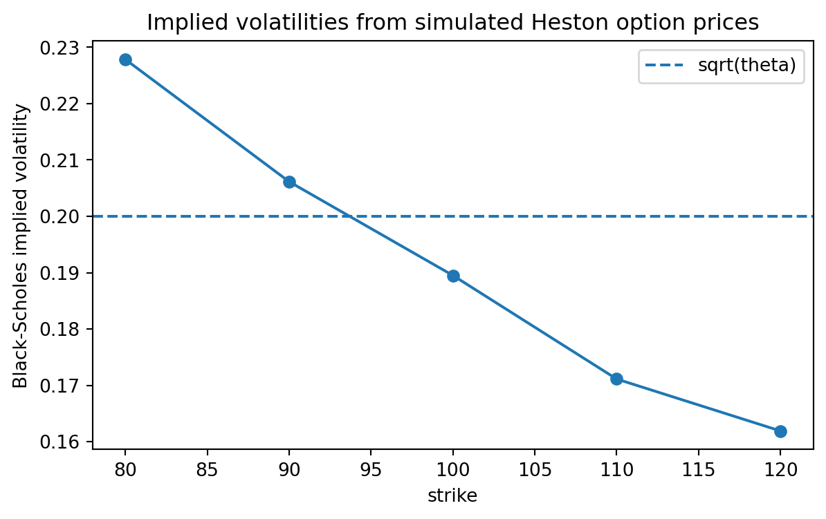

Because this is a Monte Carlo example with a modest number of paths, the smile may be noisy. Production Heston pricing usually uses Fourier methods, PDE methods, or more efficient simulation schemes.

27.29 24.24 Python Example: A Calibration Objective

Calibration means choosing model parameters so that model prices approximately match market prices. Suppose market implied volatilities are observed at several strikes. A simple least-squares objective is

\[ \min_{\Theta}\sum_i w_i \left( \sigma_{\mathrm{model}}(K_i,T_i;\Theta) - \sigma_{\mathrm{mkt}}(K_i,T_i) \right)^2. \]

market_data = pd.DataFrame({
    "K": [80, 90, 100, 110, 120],
    "T": [1, 1, 1, 1, 1],
    "market_iv": [0.29, 0.25, 0.22, 0.205, 0.20],
    "weight": [1, 1, 1, 1, 1]
})

def toy_model_iv(K, S0=100, base=0.20, rho=-0.60, xi=0.45):
    m = np.log(K / S0)
    skew = -0.18 * rho * xi
    curvature = 0.38 * xi**2
    return np.maximum(0.03, base - skew * m + curvature * m**2)

def calibration_objective(rho=-0.60, xi=0.45, base=0.20):
    model_iv = np.array([toy_model_iv(K, base=base, rho=rho, xi=xi) for K in market_data["K"]])
    residuals = model_iv - market_data["market_iv"].to_numpy()
    return np.sum(market_data["weight"].to_numpy() * residuals**2)

calibration_objective(rho=-0.60, xi=0.45, base=0.20)

0.008131402743263181

This toy function is not a Heston calibration engine. It shows the statistical structure of calibration: choose parameters, compute model quantities, compare with market quantities, and minimize weighted residuals.

27.30 24.25 Variance Swaps and Expected Integrated Variance

A variance swap pays an amount related to realized variance. In an idealized continuous-time setting, the floating leg is proportional to

\[ \frac{1}{T}\int_0^T v_t\,dt. \]

The fair variance strike is approximately

\[ K_{\mathrm{var}} = \frac{1}{T}\mathbb E^{\mathbb Q}\left[\int_0^T v_t\,dt\right]. \]

For the Heston variance process,

\[ \mathbb E^{\mathbb Q}[v_t]=\theta+(v_0-\theta)e^{-\kappa t}. \]

Therefore,

\[ \mathbb E^{\mathbb Q}\left[\int_0^T v_t\,dt\right] = \theta T+(v_0-\theta)\frac{1-e^{-\kappa T}}{\kappa}. \]

So

\[ K_{\mathrm{var}} = \theta+(v_0-\theta)\frac{1-e^{-\kappa T}}{\kappa T}. \]

def heston_expected_average_variance(v0=0.04, kappa=2.0, theta=0.04, T=1.0):
    return theta + (v0 - theta) * (1 - np.exp(-kappa * T)) / (kappa * T)

analytic_avg_var = heston_expected_average_variance(v0=v0, kappa=kappa, theta=theta, T=T)
simulated_avg_var = integrated_variance.mean() / T
analytic_avg_var, simulated_avg_var

(0.04, 0.039575661085296164)

This calculation shows that stochastic volatility models are useful not only for option pricing, but also for volatility derivatives.

27.31 24.26 Calibration: Statistics Meets Finance

Calibration is not the same as ordinary historical estimation.

Historical estimation tries to infer parameters under \(\mathbb P\) from observed time series:

\[ \{S_{t_i}\}_{i=0}^n. \]

Risk-neutral calibration tries to infer parameters under \(\mathbb Q\) from current market prices:

\[ \{C^{\mathrm{mkt}}(K_i,T_i)\}_{i=1}^m. \]

These procedures use different data and different probability measures.

For MS Statistics students, calibration can be viewed as a nonlinear inverse problem. Given a pricing map

\[ \Theta\mapsto C^{\mathrm{model}}(\Theta), \]

we choose \(\Theta\) to minimize a loss function such as

\[ L(\Theta) = \sum_{i=1}^m w_i \left(C_i^{\mathrm{model}}(\Theta)-C_i^{\mathrm{mkt}}\right)^2. \]

Important statistical issues include:

• parameter identifiability;
• noisy quotes and bid-ask spreads;
• model misspecification;
• weighting by liquidity;
• stability over time;
• overfitting to one day’s option surface.

27.32 AI-assisted calibration audit

Ask an AI assistant to review a calibration report using this checklist.

1. Does the report clearly distinguish \(\mathbb P\) parameters from \(\mathbb Q\) parameters?
2. Are market prices, implied volatilities, and bid-ask spreads specified?
3. Is the objective function written mathematically?
4. Are parameter constraints stated, including \(v_0>0\), \(\kappa>0\), \(\theta>0\), \(\xi>0\), and \(-1\le\rho\le 1\)?
5. Does the report mention whether the Feller condition is imposed?
6. Are numerical errors separated from model errors?
7. Are fitted parameters interpreted financially, not only reported numerically?

27.33 24.27 Common Mathematical Mistakes

27.34 Mistake 1: Confusing volatility and variance

In Heston, \(v_t\) is variance, not volatility. The stock diffusion coefficient is \(\sqrt{v_t}\), not \(v_t\).

27.35 Mistake 2: Forgetting the mixed derivative

When \(\rho\ne 0\), the pricing PDE contains the mixed derivative term

\[ \rho\xi vS V_{Sv}. \]

Leaving out this term changes the model.

27.36 Mistake 3: Using Euler variance without positivity correction

The Euler update can produce negative variance values. Taking \(\sqrt{v}\) after a negative update creates numerical errors or invalid values.

27.37 Mistake 4: Treating implied volatility as the model’s variance path

Implied volatility is obtained by inverting a Black–Scholes price. It is not the same object as \(\sqrt{v_t}\).

27.38 Mistake 5: Assuming no-arbitrage uniquely determines the volatility risk premium

In an incomplete stochastic volatility market, no-arbitrage alone does not determine a unique risk-neutral variance drift.

27.39 24.28 AI Component: Explaining the Heston Model Cleanly

27.40 Prompt: explain and audit notation

Explain the Heston model to MA Applied Math and MS Statistics students. Use the equations

\[ \frac{dS_t}{S_t}=r\,dt+\sqrt{v_t}\,dW_t^S, \qquad dv_t=\kappa(\theta-v_t)\,dt+\xi\sqrt{v_t}\,dW_t^v, \]

with \(d\langle W^S,W^v\rangle_t=\rho dt\). In your explanation:

• identify which variable is variance and which is volatility;
• explain mean reversion;
• explain the role of \(\rho\);
• state the Feller condition;
• explain why the model can produce an implied-volatility smile;
• identify at least three common student mistakes.

A strong AI response should make the mathematical objects precise and should not claim that the model is complete unless additional volatility-linked instruments are traded.

27.41 24.29 Summary

Stochastic volatility models extend Black–Scholes by replacing a constant variance parameter with a random variance process. The Heston model is the central example:

\[ \frac{dS_t}{S_t}=r\,dt+\sqrt{v_t}\,dW_t^S, \qquad dv_t=\kappa(\theta-v_t)\,dt+\xi\sqrt{v_t}\,dW_t^v. \]

The most important mathematical ideas are:

1. volatility is a state variable, not just a parameter;
2. the model is a two-dimensional Markov diffusion;
3. the variance process mean-reverts;
4. correlation between return and volatility shocks produces skew;
5. pricing uses risk-neutral expectation or an equivalent PDE;
6. the pricing PDE has a mixed derivative when \(\rho\ne 0\);
7. stochastic volatility markets are typically incomplete;
8. calibration is an inverse problem under the risk-neutral measure.

The core message is:

\[ \boxed{\text{Stochastic volatility = Black--Scholes with a random variance state.}} \]

27.42 24.30 Exercises

27.42.1 Conceptual exercises

1. Explain why constant-volatility Black–Scholes predicts a flat implied-volatility curve.
2. Define instantaneous variance, realized variance, and implied volatility. Explain how they differ.
3. Explain why volatility clustering motivates a stochastic volatility model.
4. In the Heston model, explain the roles of \(\kappa\), \(\theta\), \(\xi\), and \(\rho\).
5. Why is \(v_t\) called variance rather than volatility?
6. Explain why negative \(\rho\) can produce an equity-style implied-volatility skew.
7. Explain why stochastic volatility models are usually incomplete if only the stock and bond are traded.

27.42.2 Mathematical exercises

8. Use Itô’s formula to derive

\[ d\log S_t=\left(r-\frac12v_t\right)dt+\sqrt{v_t}\,dW_t^S. \]

9. Derive the expectation

\[ \mathbb E[v_t]=\theta+(v_0-\theta)e^{-\kappa t} \]

for the CIR variance process.

10. Derive

\[ \mathbb E\left[\int_0^T v_t\,dt\right] = \theta T+(v_0-\theta)\frac{1-e^{-\kappa T}}{\kappa}. \]

11. Starting from the two-dimensional Itô formula, derive the Heston pricing PDE.
12. Show explicitly where the mixed derivative term \(V_{Sv}\) enters the PDE.
13. Explain the Feller condition \(2\kappa\theta\ge \xi^2\) and what can happen when it fails.

27.42.3 Computational exercises

14. Write Python code to simulate the Heston model using full truncation Euler.
15. Compare simulated Heston paths for \(\xi=0.1\), \(\xi=0.5\), and \(\xi=1.0\).
16. Estimate the correlation between log-return increments and variance increments for several values of \(\rho\).
17. Price European calls under the Heston model by Monte Carlo for strikes \(80,90,100,110,120\).
18. Convert the prices in Exercise 17 into Black–Scholes implied volatilities.
19. Estimate the fair variance strike \(K_{\mathrm{var}}\) by simulation and compare it with the analytic expectation formula.
20. Investigate how the Monte Carlo standard error changes when the number of paths is doubled.

27.42.4 AI-assisted exercises

21. Ask an AI assistant to explain the difference between historical volatility and implied volatility. Identify any imprecise statements.
22. Ask an AI assistant to derive the Heston pricing PDE. Check carefully whether it includes the mixed derivative term.
23. Ask an AI assistant to review your Heston simulation code. Did it catch possible negative variance values?
24. Ask an AI assistant to propose a calibration objective for Heston. Rewrite the answer using precise mathematical notation.
25. Ask an AI assistant to compare Black–Scholes, local volatility, and stochastic volatility models. Turn the answer into a table with state variables, strengths, and weaknesses.