---
title: "Chapter 14. Geometric Brownian Motion"
---
::: {.chapter-objectives}
## Learning Goals
By the end of this chapter, students should be able to:
- define geometric Brownian motion as the solution of a stochastic differential equation;
- derive the explicit GBM solution using Itô's formula;
- explain why GBM keeps prices positive;
- derive the lognormal distribution of $S_t$;
- compute the mean, variance, moments, median, mode, and quantiles of a GBM price;
- distinguish arithmetic returns, log returns, drift, and volatility;
- derive conditional distributions and transition densities for GBM;
- simulate GBM exactly and compare exact simulation with Euler--Maruyama;
- estimate GBM parameters from discretely observed prices;
- understand the martingale condition for discounted GBM prices under a risk-neutral measure;
- explain the strengths and limitations of GBM as a financial model;
- use Python and AI tools to audit GBM formulas, simulations, and assumptions.
:::
::: {.hero-box}
Geometric Brownian motion is the continuous-time model
$$
dS_t=\mu S_t\,dt+\sigma S_t\,dW_t, \qquad S_0>0.
$$
Its solution is
$$
S_t=S_0\exp\left[\left(\mu-\frac12\sigma^2\right)t+\sigma W_t\right].
$$
This formula is one of the central objects in mathematical finance. It says that prices are positive, log prices are Gaussian, and multiplicative returns are driven by Brownian shocks. It also prepares the Black--Scholes model, where the physical drift $\mu$ is replaced by the risk-neutral drift $r$ for pricing.
:::
## 14.1 Why Geometric Brownian Motion?
A stock price should usually be modeled as a positive quantity. The arithmetic Brownian model
$$
dX_t=\mu\,dt+\sigma\,dW_t
$$
has normally distributed values and can become negative. This is not appropriate for a stock price, although it may be reasonable for changes in a spread or another quantity that can take both signs.
The geometric Brownian motion model makes the random shock proportional to the current price:
$$
dS_t=\mu S_t\,dt+\sigma S_t\,dW_t.
$$
Equivalently, the relative change satisfies the informal relation
$$
\frac{dS_t}{S_t}=\mu\,dt+\sigma\,dW_t.
$$
Thus the model is multiplicative rather than additive. A shock of the same Brownian size has larger dollar impact when the current price is larger.
::: {.callout-note}
## Financial interpretation
The parameter $\mu$ is the instantaneous expected return under the probability measure being used. The parameter $\sigma$ is the instantaneous volatility. Under the physical measure $\mathbb P$, $\mu$ is a statistical return parameter. Under a risk-neutral measure $\mathbb Q$, the drift of a non-dividend-paying stock becomes the risk-free rate $r$ in the Black--Scholes model.
:::
## 14.2 Definition of GBM
We work on a filtered probability space
$$
(\Omega,F,(F_t)_{t\ge 0},\mathbb P),
$$
where $W_t$ is a standard Brownian motion adapted to the filtration $(F_t)$. The filtration represents the information available through time.
::: {.definition}
### Definition 14.1: Geometric Brownian motion
A positive process $S_t$ is a geometric Brownian motion with parameters $\mu\in\mathbb R$ and $\sigma>0$ if it solves
$$
dS_t=\mu S_t\,dt+\sigma S_t\,dW_t, \qquad S_0>0.
$$
Equivalently,
$$
S_t=S_0+\int_0^t \mu S_s\,ds+\int_0^t \sigma S_s\,dW_s.
$$
:::
The second equation is the rigorous integral form. The first equation is compact differential notation.
The coefficient $\mu S_t$ is the local drift and $\sigma S_t$ is the local diffusion coefficient. Therefore, for small $\Delta t$,
$$
\mathbb E[S_{t+\Delta t}-S_t\mid F_t]\approx \mu S_t\Delta t,
$$
and
$$
\operatorname{Var}(S_{t+\Delta t}-S_t\mid F_t)\approx \sigma^2S_t^2\Delta t.
$$
Thus the conditional standard deviation of the price change is approximately
$$
\sigma S_t\sqrt{\Delta t}.
$$
This proportionality is the reason $\sigma$ is called percentage volatility.
## 14.3 Solving the GBM SDE
A common first guess is to divide by $S_t$ and integrate:
$$
\frac{dS_t}{S_t}=\mu\,dt+\sigma\,dW_t.
$$
If this were ordinary calculus, one might conclude
$$
\log S_t=\log S_0+\mu t+\sigma W_t.
$$
This is not correct. In stochastic calculus, the logarithm has an Itô correction term.
Let
$$
f(s)=\log s.
$$
Then
$$
f'(s)=\frac1s,
\qquad
f''(s)=-\frac1{s^2}.
$$
Applying Itô's formula to $S_t$ gives
$$
d\log S_t
=\frac1{S_t}\,dS_t+\frac12\left(-\frac1{S_t^2}\right)(dS_t)^2.
$$
Since
$$
dS_t=\mu S_t\,dt+\sigma S_t\,dW_t,
$$
and
$$
(dS_t)^2=\sigma^2S_t^2\,dt,
$$
we obtain
$$
d\log S_t
=\left(\mu-\frac12\sigma^2\right)dt+\sigma\,dW_t.
$$
Integrating from $0$ to $t$ yields
$$
\log S_t=\log S_0+\left(\mu-\frac12\sigma^2\right)t+\sigma W_t.
$$
Exponentiating gives the explicit solution.
::: {.theorem}
### Theorem 14.1: Explicit solution of GBM
The unique strong solution of
$$
dS_t=\mu S_t\,dt+\sigma S_t\,dW_t, \qquad S_0>0,
$$
is
$$
S_t=S_0\exp\left[\left(\mu-\frac12\sigma^2\right)t+\sigma W_t\right].
$$
In particular, $S_t>0$ for all $t\ge 0$ with probability one.
:::
::: {.proof}
Define
$$
X_t=\log S_0+\left(\mu-\frac12\sigma^2\right)t+\sigma W_t,
$$
and set $S_t=e^{X_t}$. Since
$$
dX_t=\left(\mu-\frac12\sigma^2\right)dt+\sigma\,dW_t,
$$
Itô's formula for $e^{X_t}$ gives
$$
dS_t=S_t\,dX_t+\frac12S_t(dX_t)^2.
$$
Because $(dX_t)^2=\sigma^2dt$,
$$
dS_t=S_t\left[\left(\mu-\frac12\sigma^2\right)dt+\sigma\,dW_t\right]+\frac12\sigma^2S_t\,dt.
$$
The $-\frac12\sigma^2$ and $+\frac12\sigma^2$ terms cancel, so
$$
dS_t=\mu S_t\,dt+\sigma S_t\,dW_t.
$$
Also $S_0=e^{\log S_0}$ and $S_t>0$. Standard existence and uniqueness theory for Lipschitz SDEs gives uniqueness.
:::
## 14.4 The Itô Correction Term
The term
$$
-\frac12\sigma^2t
$$
is not a modeling adjustment added by hand. It comes from quadratic variation. The differential rule is
$$
(dW_t)^2=dt.
$$
Therefore, even though the relative price equation contains drift $\mu$, the log-price drift is
$$
\mu-\frac12\sigma^2.
$$
This distinction is essential:
$$
\text{arithmetic expected return rate} = \mu,
$$
while
$$
\text{log expected return rate} = \mu-\frac12\sigma^2.
$$
::: {.callout-warning}
## Common error
The formula
$$
\log S_t=\log S_0+\mu t+\sigma W_t
$$
is missing the Itô correction. The correct formula has $\mu-\frac12\sigma^2$, not $\mu$.
:::
## 14.5 Distribution of GBM
Since $W_t\sim N(0,t)$,
$$
\log S_t\sim N\left(\log S_0+\left(\mu-\frac12\sigma^2\right)t,\sigma^2t\right).
$$
Therefore $S_t$ has a lognormal distribution.
::: {.theorem}
### Theorem 14.2: Lognormal distribution of $S_t$
For each fixed $t>0$,
$$
S_t=S_0\exp\left[\left(\mu-\frac12\sigma^2\right)t+\sigma\sqrt t Z\right],
$$
where $Z\sim N(0,1)$. Hence
$$
\log S_t\sim N\left(\log S_0+\left(\mu-\frac12\sigma^2\right)t,\sigma^2t\right).
$$
:::
The transition density of $S_t$ is
$$
p(t,s_0,s)
=
\frac{1}{s\sigma\sqrt{2\pi t}}
\exp\left[-\frac{\left(\log(s/s_0)-(\mu-\frac12\sigma^2)t\right)^2}{2\sigma^2t}\right],
\qquad s>0.
$$
This density is skewed to the right. The log price is symmetric, but the price itself is not.
## 14.6 Moments, Median, Mode, and Quantiles
A useful lognormal identity is the following. If
$$
Y\sim N(m,v),
$$
then
$$
\mathbb E[e^Y]=e^{m+v/2}.
$$
For GBM,
$$
Y=\log S_t.
$$
Thus
$$
\mathbb E[S_t]
=S_0e^{\mu t}.
$$
The second moment is
$$
\mathbb E[S_t^2]
=S_0^2e^{2\mu t+\sigma^2t}.
$$
Therefore
$$
\operatorname{Var}(S_t)
=S_0^2e^{2\mu t}\left(e^{\sigma^2t}-1\right).
$$
More generally, for any real $p$,
$$
\mathbb E[S_t^p]
=S_0^p\exp\left[p\mu t+\frac12p(p-1)\sigma^2t\right].
$$
The median is
$$
\operatorname{Median}(S_t)=S_0\exp\left[\left(\mu-\frac12\sigma^2\right)t\right],
$$
and the mode is
$$
\operatorname{Mode}(S_t)=S_0\exp\left[\left(\mu-\frac32\sigma^2\right)t\right].
$$
The $\alpha$-quantile is
$$
q_\alpha(t)
=S_0\exp\left[\left(\mu-\frac12\sigma^2\right)t+\sigma\sqrt t\,z_\alpha\right],
$$
where $z_\alpha$ is the $\alpha$-quantile of the standard normal distribution.
::: {.callout-tip}
## Mean versus median
For $\sigma>0$,
$$
\operatorname{Median}(S_t)<\mathbb E[S_t].
$$
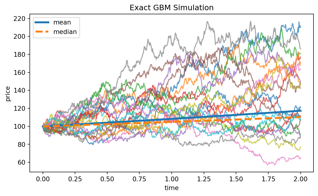
This is a feature of the right-skewed lognormal distribution. In simulations, many paths can finish below the mean even when the expected price is high.
:::
## 14.7 Interactive Demo: GBM Paths
The following activity shows how drift and volatility affect sample paths. Increasing $\mu$ raises the average growth. Increasing $\sigma$ spreads the paths and also lowers the median growth rate because the log drift is $\mu-\frac12\sigma^2$.
::: {.interactive-card}
### Interactive: Simulated GBM paths
Use the sliders to change $\mu$ and $\sigma$. The demo uses exact GBM updates and local Plotly.js.
<div class="mf-controls">
<label for="ch14-gbm-mu">Drift mu</label>
<input id="ch14-gbm-mu" type="range" min="-0.10" max="0.25" value="0.08" step="0.01">
<span id="ch14-gbm-mu-value">0.08</span>
<label for="ch14-gbm-sigma">Volatility sigma</label>
<input id="ch14-gbm-sigma" type="range" min="0.05" max="0.80" value="0.25" step="0.01">
<span id="ch14-gbm-sigma-value">0.25</span>
</div>
<div id="ch14-gbm-path-demo" class="plotly-demo"></div>
<script>
window.mfPlotlyReady(function() {
var el = document.getElementById("ch14-gbm-path-demo");
if (!el) return;
var muSlider = document.getElementById("ch14-gbm-mu");
var sigmaSlider = document.getElementById("ch14-gbm-sigma");
var muValue = document.getElementById("ch14-gbm-mu-value");
var sigmaValue = document.getElementById("ch14-gbm-sigma-value");
function normalRandom() {
var u = 0, v = 0;
while (u === 0) u = Math.random();
while (v === 0) v = Math.random();
return Math.sqrt(-2.0 * Math.log(u)) * Math.cos(2.0 * Math.PI * v);
}
function draw() {
var mu = parseFloat(muSlider.value);
var sigma = parseFloat(sigmaSlider.value);
muValue.textContent = mu.toFixed(2);
sigmaValue.textContent = sigma.toFixed(2);
var S0 = 100.0;
var T = 2.0;
var n = 240;
var dt = T / n;
var t = Array.from({length: n + 1}, function(_, i) { return i * dt; });
var traces = [];
for (var path = 0; path < 30; path++) {
var s = S0;
var y = [s];
for (var i = 1; i <= n; i++) {
var z = normalRandom();
s = s * Math.exp((mu - 0.5 * sigma * sigma) * dt + sigma * Math.sqrt(dt) * z);
y.push(s);
}
traces.push({x: t, y: y, mode: "lines", line: {width: 1}, opacity: 0.50, showlegend: false});
}
traces.push({
x: t,
y: t.map(function(x) { return S0 * Math.exp(mu * x); }),
mode: "lines",
name: "mean: S0 exp(mu t)",
line: {width: 4}
});
traces.push({
x: t,
y: t.map(function(x) { return S0 * Math.exp((mu - 0.5 * sigma * sigma) * x); }),
mode: "lines",
name: "median",
line: {width: 4, dash: "dash"}
});
Plotly.react(el, traces, {
title: "Geometric Brownian Motion Sample Paths",
xaxis: {title: "time"},
yaxis: {title: "price"},
margin: {l: 60, r: 20, t: 50, b: 50}
}, {responsive: true});
}
muSlider.addEventListener("input", draw);
sigmaSlider.addEventListener("input", draw);
draw();
});
</script>
:::
## 14.8 Python Example: Simulating GBM Exactly
The exact discretization follows directly from the solution. For a time step $\Delta t$,
$$
S_{t+\Delta t}=S_t\exp\left[\left(\mu-\frac12\sigma^2\right)\Delta t+\sigma\sqrt{\Delta t}Z\right],
$$
where $Z\sim N(0,1)$.
```{python}
import numpy as np
import matplotlib.pyplot as plt

rng = np.random.default_rng(7243)

S0 = 100.0
mu = 0.08
sigma = 0.25
T = 2.0
n_steps = 500
n_paths = 20

dt = T / n_steps
time = np.linspace(0.0, T, n_steps + 1)

Z = rng.normal(size=(n_paths, n_steps))
log_increments = (mu - 0.5 * sigma**2) * dt + sigma * np.sqrt(dt) * Z
log_paths = np.cumsum(log_increments, axis=1)
S = np.empty((n_paths, n_steps + 1))
S[:, 0] = S0
S[:, 1:] = S0 * np.exp(log_paths)

plt.figure(figsize=(8, 4.5))
for j in range(n_paths):
    plt.plot(time, S[j], alpha=0.7)
plt.plot(time, S0 * np.exp(mu * time), linewidth=3, label="mean")
plt.plot(time, S0 * np.exp((mu - 0.5 * sigma**2) * time), linewidth=3, linestyle="--", label="median")
plt.xlabel("time")
plt.ylabel("price")
plt.title("Exact GBM Simulation")
plt.legend()
plt.show()
```
The simulation uses independent normal shocks. The same formula is used in Monte Carlo pricing and risk simulation.
## 14.9 Arithmetic Returns and Log Returns
For discrete observations $0=t_0<t_1<\cdots<t_n$, define the simple return
$$
R_i=\frac{S_{t_i}-S_{t_{i-1}}}{S_{t_{i-1}}},
$$
and the log return
$$
r_i=\log\frac{S_{t_i}}{S_{t_{i-1}}}.
$$
Under GBM with equally spaced step $\Delta t$,
$$
r_i\sim N\left(\left(\mu-\frac12\sigma^2\right)\Delta t,\sigma^2\Delta t\right),
$$
and the $r_i$ are independent.
The simple return satisfies
$$
1+R_i=e^{r_i}.
$$
Therefore $R_i$ is shifted lognormal. Its conditional expected value is
$$
\mathbb E[R_i]=e^{\mu\Delta t}-1.
$$
For small $\Delta t$,
$$
e^{\mu\Delta t}-1\approx \mu\Delta t.
$$
::: {.callout-note}
## Why log returns are convenient
Log returns are additive:
$$
\log\frac{S_T}{S_0}=\sum_{i=1}^n \log\frac{S_{t_i}}{S_{t_{i-1}}}.
$$
This additivity is why log returns are mathematically convenient. Simple returns are easier to interpret as percentage gains or losses, but they are not additive across time.
:::
```{python}
# Distribution of one-period log returns under GBM
rng = np.random.default_rng(123)

mu = 0.08
sigma = 0.25
dt = 1 / 252
n = 50_000

log_returns = (mu - 0.5 * sigma**2) * dt + sigma * np.sqrt(dt) * rng.normal(size=n)
simple_returns = np.exp(log_returns) - 1

print("Sample mean log return:", log_returns.mean())
print("Theoretical mean log return:", (mu - 0.5 * sigma**2) * dt)
print("Sample variance log return:", log_returns.var(ddof=1))
print("Theoretical variance log return:", sigma**2 * dt)
print("Sample mean simple return:", simple_returns.mean())
print("Theoretical mean simple return:", np.exp(mu * dt) - 1)
```
## 14.10 Conditional Distribution and Markov Property
GBM is a Markov process. Given $S_t$, the future depends only on the current value and independent Brownian increments. For $u>t$,
$$
S_u=S_t\exp\left[\left(\mu-\frac12\sigma^2\right)(u-t)+\sigma(W_u-W_t)\right].
$$
Since
$$
W_u-W_t\sim N(0,u-t)
$$
and is independent of $F_t$, we have
$$
\log S_u\mid F_t
\sim
N\left(\log S_t+\left(\mu-\frac12\sigma^2\right)(u-t),\sigma^2(u-t)\right).
$$
Consequently,
$$
\mathbb E[S_u\mid F_t]=S_te^{\mu(u-t)}.
$$
This conditional expectation is useful for forecasting under $\mathbb P$, but pricing derivatives requires risk-neutral expectations under $\mathbb Q$.
::: {.theorem}
### Theorem 14.3: Markov transition of GBM
For $0\le t<u$ and $s>0$,
$$
S_u\mid S_t=s
\overset{d}{=}
s\exp\left[\left(\mu-\frac12\sigma^2\right)(u-t)+\sigma\sqrt{u-t}Z\right],
$$
where $Z\sim N(0,1)$.
:::
## 14.11 Interactive Demo: Terminal Lognormal Distribution
The terminal distribution of $S_T$ changes shape as $\sigma$ changes. The log price remains normal, but the price distribution becomes more right-skewed.
::: {.interactive-card}
### Interactive: Lognormal terminal distribution
The plot shows the density of $S_T$ for a GBM model.
<div class="mf-controls">
<label for="ch14-density-sigma">Volatility sigma</label>
<input id="ch14-density-sigma" type="range" min="0.05" max="0.80" value="0.25" step="0.01">
<span id="ch14-density-sigma-value">0.25</span>
<label for="ch14-density-T">Maturity T</label>
<input id="ch14-density-T" type="range" min="0.25" max="5.00" value="1.00" step="0.25">
<span id="ch14-density-T-value">1.00</span>
</div>
<div id="ch14-lognormal-density-demo" class="plotly-demo"></div>
<script>
window.mfPlotlyReady(function() {
var el = document.getElementById("ch14-lognormal-density-demo");
if (!el) return;
var sigmaSlider = document.getElementById("ch14-density-sigma");
var TSlider = document.getElementById("ch14-density-T");
var sigmaValue = document.getElementById("ch14-density-sigma-value");
var TValue = document.getElementById("ch14-density-T-value");
function normalCdfApprox(x) {
var t = 1 / (1 + 0.2316419 * Math.abs(x));
var d = 0.3989423 * Math.exp(-x * x / 2);
var prob = d * t * (0.3193815 + t * (-0.3565638 + t * (1.781478 + t * (-1.821256 + t * 1.330274))));
return x > 0 ? 1 - prob : prob;
}
function draw() {
var S0 = 100.0;
var mu = 0.08;
var sigma = parseFloat(sigmaSlider.value);
var T = parseFloat(TSlider.value);
sigmaValue.textContent = sigma.toFixed(2);
TValue.textContent = T.toFixed(2);
var m = Math.log(S0) + (mu - 0.5 * sigma * sigma) * T;
var v = sigma * sigma * T;
var sd = Math.sqrt(v);
var lo = Math.max(1, S0 * Math.exp((mu - 0.5 * sigma * sigma) * T - 4 * sigma * Math.sqrt(T)));
var hi = S0 * Math.exp((mu - 0.5 * sigma * sigma) * T + 4 * sigma * Math.sqrt(T));
var x = [];
var y = [];
var n = 300;
for (var i = 0; i < n; i++) {
var s = lo + (hi - lo) * i / (n - 1);
var dens = Math.exp(-Math.pow(Math.log(s) - m, 2) / (2 * v)) / (s * sd * Math.sqrt(2 * Math.PI));
x.push(s);
y.push(dens);
}
var mean = S0 * Math.exp(mu * T);
var median = S0 * Math.exp((mu - 0.5 * sigma * sigma) * T);
var probBelowS0 = normalCdfApprox((Math.log(S0) - m) / sd);
var traces = [
{x: x, y: y, mode: "lines", name: "density", line: {width: 3}},
{x: [mean, mean], y: [0, Math.max.apply(null, y)], mode: "lines", name: "mean", line: {dash: "dash", width: 3}},
{x: [median, median], y: [0, Math.max.apply(null, y)], mode: "lines", name: "median", line: {dash: "dot", width: 3}}
];
Plotly.react(el, traces, {
title: "Terminal GBM Density; P(S_T < S0) approx " + probBelowS0.toFixed(3),
xaxis: {title: "terminal price S(T)"},
yaxis: {title: "density"},
margin: {l: 60, r: 20, t: 60, b: 50}
}, {responsive: true});
}
sigmaSlider.addEventListener("input", draw);
TSlider.addEventListener("input", draw);
draw();
});
</script>
:::
## 14.12 Moment Generating Structure of Log Prices
The log price is Gaussian, so it has a simple moment generating function. Let
$$
X_t=\log\frac{S_t}{S_0}.
$$
Then
$$
X_t=\left(\mu-\frac12\sigma^2\right)t+\sigma W_t.
$$
For any real $u$,
$$
\mathbb E[e^{uX_t}]
=
\exp\left[u\left(\mu-\frac12\sigma^2\right)t+\frac12u^2\sigma^2t\right].
$$
This identity is a compact way to recover all power moments of $S_t$ because
$$
S_t^u=S_0^u e^{uX_t}.
$$
It is also the starting point for characteristic-function methods in more advanced models.
## 14.13 The Generator of GBM
For a twice differentiable test function $f$, Itô's formula gives
$$
df(S_t)
=\left(\mu S_t f'(S_t)+\frac12\sigma^2S_t^2f''(S_t)\right)dt
+\sigma S_t f'(S_t)\,dW_t.
$$
The infinitesimal generator of GBM is therefore
$$
L f(s)=\mu s f'(s)+\frac12\sigma^2s^2 f''(s).
$$
The generator is important because it connects stochastic processes with PDEs. If
$$
u(t,s)=\mathbb E[g(S_T)\mid S_t=s],
$$
then, under regularity conditions, $u$ satisfies the backward equation
$$
u_t+L u=0,
\qquad
u(T,s)=g(s).
$$
In the Black--Scholes model, the same generator appears with drift $r$ under the risk-neutral measure, and discounting contributes an extra term $-ru$.
```{python}
# Generator check for f(s) = s^p
import sympy as sp

s, mu_sym, sigma_sym, p = sp.symbols("s mu sigma p", positive=True)
f = s**p
Lf = mu_sym * s * sp.diff(f, s) + sp.Rational(1, 2) * sigma_sym**2 * s**2 * sp.diff(f, s, 2)
sp.factor(Lf)
```
For $f(s)=s^p$,
$$
L f(s)=\left[p\mu+\frac12p(p-1)\sigma^2\right]s^p.
$$
This agrees with the moment formula.
## 14.14 Discounted GBM and Martingales
Let the money-market account be
$$
B_t=e^{rt}.
$$
If a stock follows
$$
dS_t=\mu S_t\,dt+\sigma S_t\,dW_t
$$
under the physical measure $\mathbb P$, then the discounted stock is
$$
\widetilde S_t=e^{-rt}S_t.
$$
By the product rule,
$$
d\widetilde S_t=(\mu-r)\widetilde S_t\,dt+\sigma\widetilde S_t\,dW_t.
$$
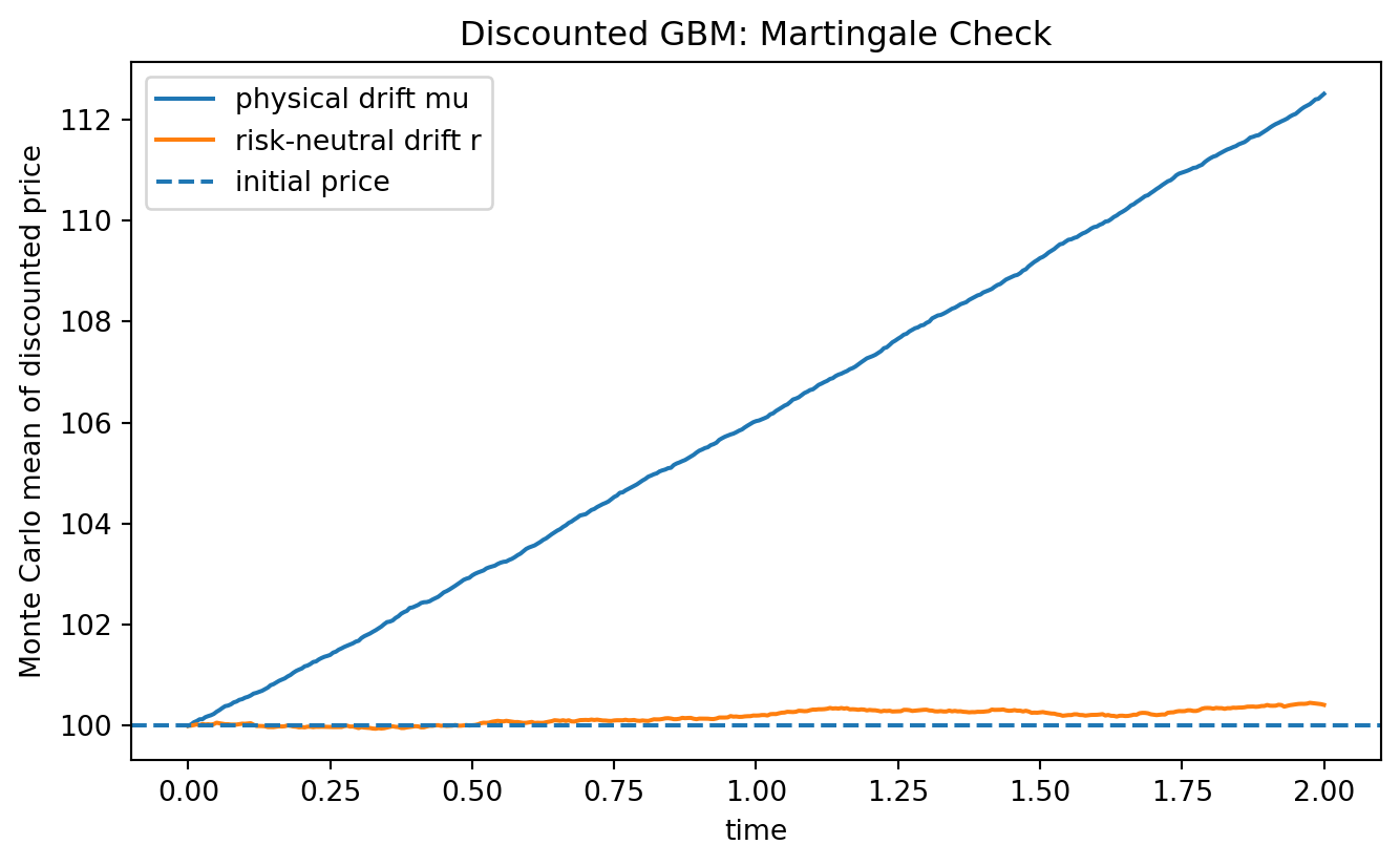
Thus $\widetilde S_t$ is generally not a martingale under $\mathbb P$ unless $\mu=r$.
Under a risk-neutral measure $\mathbb Q$ for a non-dividend-paying stock, the stock dynamics are
$$
dS_t=rS_t\,dt+\sigma S_t\,dW_t^{\mathbb Q}.
$$
Then
$$
d(e^{-rt}S_t)=\sigma e^{-rt}S_t\,dW_t^{\mathbb Q},
$$
so the discounted stock is a martingale under $\mathbb Q$.
::: {.callout-important}
## Pricing versus forecasting
The physical drift $\mu$ is relevant for forecasting under $\mathbb P$. The risk-neutral drift $r$ is relevant for no-arbitrage pricing under $\mathbb Q$. The volatility $\sigma$ appears in both. This distinction is one of the main conceptual steps from stochastic modeling to derivative pricing.
:::
## 14.15 Python Example: Discounted Martingale Check
The following simulation compares discounted GBM under physical drift $\mu$ and risk-neutral drift $r$.
```{python}
rng = np.random.default_rng(2026)

S0 = 100.0
r = 0.04
mu = 0.10
sigma = 0.25
T = 2.0
n_steps = 400
n_paths = 30_000

dt = T / n_steps
time = np.linspace(0.0, T, n_steps + 1)

def simulate_gbm_paths(drift):
    Z = rng.normal(size=(n_paths, n_steps))
    increments = (drift - 0.5 * sigma**2) * dt + sigma * np.sqrt(dt) * Z
    log_paths = np.cumsum(increments, axis=1)
    S = np.empty((n_paths, n_steps + 1))
    S[:, 0] = S0
    S[:, 1:] = S0 * np.exp(log_paths)
    return S

S_physical = simulate_gbm_paths(mu)
S_risk_neutral = simulate_gbm_paths(r)

disc = np.exp(-r * time)
mean_disc_physical = (S_physical * disc).mean(axis=0)
mean_disc_risk_neutral = (S_risk_neutral * disc).mean(axis=0)

plt.figure(figsize=(8, 4.5))
plt.plot(time, mean_disc_physical, label="physical drift mu")
plt.plot(time, mean_disc_risk_neutral, label="risk-neutral drift r")
plt.axhline(S0, linestyle="--", label="initial price")
plt.xlabel("time")
plt.ylabel("Monte Carlo mean of discounted price")
plt.title("Discounted GBM: Martingale Check")
plt.legend()
plt.show()

print("Final discounted mean under physical drift:", mean_disc_physical[-1])
print("Final discounted mean under risk-neutral drift:", mean_disc_risk_neutral[-1])
```
The risk-neutral discounted mean should stay close to $S_0$. The physical discounted mean grows when $\mu>r$.
## 14.16 Exact Simulation versus Euler--Maruyama
Euler--Maruyama applied to GBM gives
$$
S_{n+1}^{E}=S_n^E+\mu S_n^E\Delta t+\sigma S_n^E\sqrt{\Delta t}Z_{n+1}.
$$
Equivalently,
$$
S_{n+1}^{E}=S_n^E\left(1+\mu\Delta t+\sigma\sqrt{\Delta t}Z_{n+1}\right).
$$
This approximation can become negative if the factor in parentheses is negative. The exact update is
$$
S_{n+1}=S_n\exp\left[\left(\mu-\frac12\sigma^2\right)\Delta t+\sigma\sqrt{\Delta t}Z_{n+1}\right],
$$
which always stays positive.
::: {.callout-warning}
## Simulation warning
For GBM, use the exact update when possible. Euler--Maruyama is important for general SDEs, but for GBM it can introduce artificial negative prices.
:::
```{python}
rng = np.random.default_rng(77)

S0 = 100.0
mu = 0.05
sigma = 0.80
T = 1.0
n_steps = 12
n_paths = 100_000

dt = T / n_steps
Z = rng.normal(size=(n_paths, n_steps))

S_exact = np.full(n_paths, S0)
S_euler = np.full(n_paths, S0)

for k in range(n_steps):
    S_exact *= np.exp((mu - 0.5 * sigma**2) * dt + sigma * np.sqrt(dt) * Z[:, k])
    S_euler *= 1 + mu * dt + sigma * np.sqrt(dt) * Z[:, k]

negative_rate = np.mean(S_euler <= 0)
print("Fraction of Euler terminal values <= 0:", negative_rate)
print("Minimum exact terminal value:", S_exact.min())
print("Minimum Euler terminal value:", S_euler.min())
```
## 14.17 Parameter Estimation from Log Returns
Suppose prices are observed at equally spaced times with step $\Delta t$. The GBM log returns satisfy
$$
r_i=\log\frac{S_{t_i}}{S_{t_{i-1}}}
=\left(\mu-\frac12\sigma^2\right)\Delta t+\sigma\sqrt{\Delta t}Z_i.
$$
Thus
$$
\bar r\approx \left(\mu-\frac12\sigma^2\right)\Delta t,
$$
and
$$
s_r^2\approx \sigma^2\Delta t.
$$
A natural estimator is
$$
\widehat\sigma=\frac{s_r}{\sqrt{\Delta t}},
$$
and
$$
\widehat\mu=\frac{\bar r}{\Delta t}+\frac12\widehat\sigma^2.
$$
```{python}
rng = np.random.default_rng(2027)

S0 = 100.0
mu_true = 0.09
sigma_true = 0.22
T = 5.0
steps_per_year = 252
n_steps = int(T * steps_per_year)
dt = 1 / steps_per_year

Z = rng.normal(size=n_steps)
log_r = (mu_true - 0.5 * sigma_true**2) * dt + sigma_true * np.sqrt(dt) * Z
prices = S0 * np.exp(np.cumsum(np.r_[0.0, log_r]))

sample_mean = log_r.mean()
sample_std = log_r.std(ddof=1)

sigma_hat = sample_std / np.sqrt(dt)
mu_hat = sample_mean / dt + 0.5 * sigma_hat**2

print("True mu:", mu_true)
print("Estimated mu:", mu_hat)
print("True sigma:", sigma_true)
print("Estimated sigma:", sigma_hat)
```
The volatility estimate is usually more stable than the drift estimate. This is one reason financial forecasting is difficult: expected returns are hard to estimate from noisy returns.
::: {.callout-note}
## Statistical warning
Even in the ideal GBM model, estimating $\mu$ accurately requires a large amount of data. Volatility is easier to estimate because it is tied to second-order variation. This connects to quadratic variation in continuous time.
:::
## 14.18 Likelihood for Discrete GBM Observations
Let
$$
r_i=\log\frac{S_{t_i}}{S_{t_{i-1}}}.
$$
Under GBM,
$$
r_i\sim N(m\Delta t,\sigma^2\Delta t),
\qquad
m=\mu-\frac12\sigma^2.
$$
The log-likelihood for $m$ and $\sigma$ is
$$
\ell(m,\sigma)
=-\frac n2\log(2\pi\sigma^2\Delta t)
-\frac{1}{2\sigma^2\Delta t}\sum_{i=1}^n(r_i-m\Delta t)^2.
$$
The maximum likelihood estimator of $m$ is
$$
\widehat m=\frac{\bar r}{\Delta t},
$$
and the maximum likelihood estimator of $\sigma^2$ is
$$
\widehat\sigma^2_{MLE}
=\frac1{n\Delta t}\sum_{i=1}^n(r_i-\bar r)^2.
$$
Then
$$
\widehat\mu=\widehat m+\frac12\widehat\sigma^2_{MLE}.
$$
Notice that this differs slightly from the unbiased sample variance formula because maximum likelihood uses $1/n$ rather than $1/(n-1)$.
## 14.19 GBM and European Option Payoffs
GBM gives the terminal stock model used in the Black--Scholes formula. Under the risk-neutral measure,
$$
S_T=S_0\exp\left[\left(r-\frac12\sigma^2\right)T+\sigma\sqrt T Z\right].
$$
A European call with strike $K$ has payoff
$$
(S_T-K)^+.
$$
The no-arbitrage price is
$$
C_0=e^{-rT}\mathbb E^{\mathbb Q}[(S_T-K)^+].
$$
The closed-form evaluation appears in Chapter 16. For now, GBM already gives a Monte Carlo pricing method.
```{python}
rng = np.random.default_rng(88)

S0 = 100.0
K = 105.0
r = 0.04
sigma = 0.25
T = 1.0
n = 200_000

Z = rng.normal(size=n)
S_T = S0 * np.exp((r - 0.5 * sigma**2) * T + sigma * np.sqrt(T) * Z)
payoff = np.maximum(S_T - K, 0.0)
price_mc = np.exp(-r * T) * payoff.mean()
standard_error = np.exp(-r * T) * payoff.std(ddof=1) / np.sqrt(n)

print("Monte Carlo call price:", price_mc)
print("Monte Carlo standard error:", standard_error)
```
This method is conceptually simple: simulate terminal prices under $\mathbb Q$, compute payoffs, average, and discount.
## 14.20 Time Scaling and Annualization
If $r_i$ denotes a daily log return and there are approximately $252$ trading days in a year, GBM suggests the scaling rules
$$
\operatorname{Mean annual log return}\approx 252\cdot \operatorname{Mean daily log return},
$$
and
$$
\operatorname{Annual volatility}\approx \sqrt{252}\cdot \operatorname{Daily volatility}.
$$
The second rule comes from variance additivity for independent log returns:
$$
\operatorname{Var}\left(\sum_{i=1}^{252}r_i\right)
=252\operatorname{Var}(r_1).
$$
These rules rely on independence and constant volatility. Real returns often have volatility clustering, so the square-root-of-time rule should be treated as a model-based approximation.
## 14.21 GBM as an Exponential Martingale
The process
$$
M_t=\exp\left(\sigma W_t-\frac12\sigma^2t\right)
$$
is a martingale. GBM can be written as
$$
S_t=S_0e^{\mu t}M_t.
$$
Therefore
$$
\mathbb E[S_t]=S_0e^{\mu t}\mathbb E[M_t]=S_0e^{\mu t}.
$$
This representation separates deterministic growth from stochastic martingale fluctuation.
::: {.theorem}
### Theorem 14.4: Exponential martingale representation
For fixed $\sigma$, the process
$$
M_t=\exp\left(\sigma W_t-\frac12\sigma^2t\right)
$$
is a martingale with $\mathbb E[M_t]=1$. GBM satisfies
$$
S_t=S_0e^{\mu t}M_t.
$$
:::
::: {.proof}
For $0\le s<t$,
$$
M_t=M_s\exp\left(\sigma(W_t-W_s)-\frac12\sigma^2(t-s)\right).
$$
The increment $W_t-W_s$ is independent of $F_s$ and is normally distributed with variance $t-s$. Hence
$$
\mathbb E\left[\exp\left(\sigma(W_t-W_s)-\frac12\sigma^2(t-s)\right)\mid F_s\right]=1.
$$
Therefore
$$
\mathbb E[M_t\mid F_s]=M_s.
$$
:::
## 14.22 Model Strengths and Limitations
GBM is mathematically elegant and financially useful, but it is not a complete description of real markets.
### Strengths
1. **Positivity.** Prices remain positive.
2. **Analytic tractability.** Log prices are Gaussian and many quantities have closed forms.
3. **Markov structure.** Conditional distributions are simple.
4. **Exact simulation.** No discretization error is needed for simulation at fixed dates.
5. **Black--Scholes foundation.** It leads to the classical option-pricing model.
### Limitations
1. **Constant volatility.** Real market volatility changes over time.
2. **No jumps.** GBM paths are continuous, while markets can move abruptly.
3. **Lognormal tails.** Real returns often show heavier tails than the normal log-return assumption.
4. **No volatility smile.** The Black--Scholes model based on GBM cannot explain all observed option prices with one constant volatility.
5. **Uncertain drift.** Expected returns are difficult to estimate.
6. **Independent increments.** Real returns may show dependence in volatility even when returns themselves have weak autocorrelation.
These limitations motivate later chapters on stochastic volatility, jump models, and model risk.
## 14.23 Python Example: A Simple GBM Diagnostic Workflow
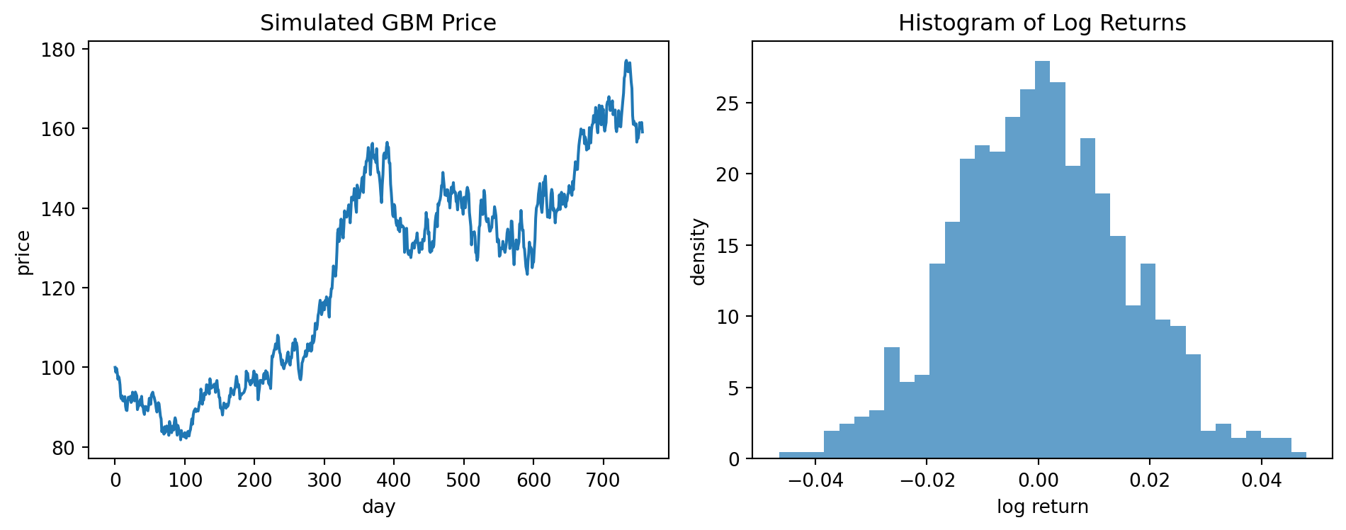
The following workflow simulates data from GBM and checks whether the log returns look approximately normal and independent.
```{python}
rng = np.random.default_rng(909)

S0 = 100.0
mu = 0.08
sigma = 0.25
steps_per_year = 252
T = 3.0
n_steps = int(T * steps_per_year)
dt = 1 / steps_per_year

log_r = (mu - 0.5 * sigma**2) * dt + sigma * np.sqrt(dt) * rng.normal(size=n_steps)
prices = S0 * np.exp(np.cumsum(np.r_[0.0, log_r]))

fig, axes = plt.subplots(1, 2, figsize=(10, 4))
axes[0].plot(prices)
axes[0].set_title("Simulated GBM Price")
axes[0].set_xlabel("day")
axes[0].set_ylabel("price")

axes[1].hist(log_r, bins=35, density=True, alpha=0.7)
axes[1].set_title("Histogram of Log Returns")
axes[1].set_xlabel("log return")
axes[1].set_ylabel("density")
plt.tight_layout()
plt.show()

lag1_corr = np.corrcoef(log_r[:-1], log_r[1:])[0, 1]
print("Lag-1 sample correlation of log returns:", lag1_corr)
```
In real data, the histogram and correlations should be treated as diagnostics, not proof. A model can be useful even when it is not literally true.
## 14.24 AI-Assisted Learning Components
AI tools are useful for checking derivations and code, but students should verify all formulas independently.
::: {.callout-tip}
## AI prompt: Audit the GBM solution
Ask an AI assistant:
> Derive the solution of $dS_t=\mu S_tdt+\sigma S_tdW_t$ using Itô's formula. Explain why the log drift is $\mu-\frac12\sigma^2$, not $\mu$.
Then check whether the response explicitly uses the second derivative of $\log s$ and the rule $(dW_t)^2=dt$.
:::
::: {.callout-tip}
## AI prompt: Check simulation code
Give an AI assistant your GBM simulation code and ask:
> Does this code simulate GBM exactly or by Euler--Maruyama? Does it use the term $(\mu-\frac12\sigma^2)\Delta t$ in the exponent? Can the simulated prices become negative?
Then verify the answer by inspecting the update formula.
:::
::: {.callout-tip}
## AI prompt: Critique the model
Ask:
> What assumptions of geometric Brownian motion are unrealistic for financial returns? Which later models relax each assumption?
A strong answer should mention constant volatility, continuous paths, normal log returns, independent increments, and volatility smiles.
:::
## 14.25 Common Mistakes
1. **Forgetting the Itô correction.** The log drift is $\mu-\frac12\sigma^2$, not $\mu$.
2. **Confusing $\mu$ with the log-return mean.** The parameter $\mu$ is the arithmetic expected return rate.
3. **Confusing physical and risk-neutral drift.** Use $\mu$ for statistical modeling under $\mathbb P$ and $r$ for risk-neutral pricing under $\mathbb Q$ in the basic Black--Scholes setting.
4. **Assuming mean and median are the same.** The lognormal distribution is skewed.
5. **Using Euler when exact simulation is available.** Euler can produce negative prices.
6. **Treating annualization as a law of nature.** Square-root-of-time volatility scaling is model-based.
7. **Estimating drift too confidently.** Drift estimation is noisy.
8. **Assuming GBM is empirically perfect.** GBM is a foundational model, not a complete model of markets.
## 14.26 Exercises
### Conceptual Exercises
1. Explain why GBM is a multiplicative model rather than an additive model.
2. Why does GBM preserve positivity?
3. Explain the difference between the drift of $S_t$ and the drift of $\log S_t$.
4. Why is $S_t$ lognormal but $\log S_t$ normal?
5. Explain why $\mathbb E[S_t]$ is larger than the median of $S_t$ when $\sigma>0$.
6. In the Black--Scholes model, why does the risk-neutral stock drift equal $r$ rather than $\mu$?
### Mathematical Exercises
7. Use Itô's formula to prove the GBM solution formula.
8. Derive $\mathbb E[S_t]$ and $\operatorname{Var}(S_t)$.
9. Show that for real $p$,
$$
\mathbb E[S_t^p]
=S_0^p\exp\left[p\mu t+\frac12p(p-1)\sigma^2t\right].
$$
10. Derive the transition density of $S_t$ given $S_0=s_0$.
11. Prove that
$$
M_t=\exp\left(\sigma W_t-\frac12\sigma^2t\right)
$$
is a martingale.
12. Compute the generator $L$ of GBM and evaluate $Lf$ for $f(s)=s$, $f(s)=s^2$, and $f(s)=\log s$.
13. Show that under risk-neutral GBM,
$$
\mathbb E^{\mathbb Q}[e^{-rT}S_T]=S_0.
$$
### Computational Exercises
14. Simulate exact GBM paths for several values of $\sigma$. Plot the mean and median curves.
15. Compare exact GBM simulation with Euler--Maruyama for large $\sigma$ and coarse time steps.
16. Estimate $\mu$ and $\sigma$ from simulated daily prices. Repeat the experiment many times and compare the variability of the two estimators.
17. Simulate $S_T$ and compare the empirical mean, variance, median, and 5 percent quantile with theoretical values.
18. Use Monte Carlo simulation under risk-neutral GBM to estimate a European put price.
19. For simulated GBM log returns, make a histogram and QQ plot. Explain what pattern you expect.
### AI-Assisted Exercises
20. Ask an AI assistant to derive the GBM density. Check whether it correctly applies the change-of-variables formula from normal to lognormal.
21. Ask an AI assistant to explain why Euler--Maruyama can produce negative values for GBM. Rewrite the explanation using the exact update formula.
22. Ask an AI assistant to compare GBM with a jump-diffusion model. Identify which GBM assumptions are changed.
23. Ask an AI assistant to generate code for estimating $\mu$ and $\sigma$ from log returns. Check whether the time step $\Delta t$ is handled correctly.
24. Ask an AI assistant whether GBM is a martingale. Explain why the precise answer depends on whether we mean $S_t$, $e^{-rt}S_t$, and which probability measure is being used.
## 14.27 Chapter Summary
Geometric Brownian motion is the positive continuous-time price model
$$
dS_t=\mu S_t\,dt+\sigma S_t\,dW_t.
$$
Its solution is
$$
S_t=S_0\exp\left[\left(\mu-\frac12\sigma^2\right)t+\sigma W_t\right].
$$
The Itô correction term $-\frac12\sigma^2$ is the key mathematical feature. It implies that log returns are normally distributed with mean $\left(\mu-\frac12\sigma^2\right)t$ and variance $\sigma^2t$, while prices are lognormal. GBM gives exact simulation formulas, transition densities, moment formulas, and a simple Markov structure. Under a risk-neutral measure, replacing $\mu$ by $r$ makes the discounted stock price a martingale. This prepares the Black--Scholes model and formula in the next chapters. At the same time, GBM's constant volatility, continuous paths, and normal log returns are strong assumptions, motivating more advanced models later in the book.