---
title: "Chapter 3. One-Period Asset Pricing"
---
::: {.chapter-objectives}
## Learning Goals
By the end of this chapter, students should be able to:
- formulate a one-period financial market on a finite state space;
- represent assets, portfolios, and derivative claims using vectors and matrices;
- define arbitrage, no-arbitrage, attainable claims, and market completeness;
- prove the law of one price from the no-arbitrage condition;
- derive state prices as positive linear pricing weights;
- convert state prices into risk-neutral probabilities when a riskless asset is present;
- price one-period derivative claims by replication and by risk-neutral expectation;
- distinguish physical probabilities from pricing probabilities;
- compute no-arbitrage price bounds for unattainable claims in incomplete markets;
- implement one-period asset-pricing calculations in Python;
- use AI tools responsibly to check definitions, assumptions, algebra, and code.
:::
::: {.hero-box}
One-period asset pricing is the finite-dimensional prototype of the whole book.
A market gives us **prices today** and **payoffs tomorrow**. The no-arbitrage principle asks whether these objects can coexist without creating a free profit. If they can, then prices can be represented by positive state prices, or equivalently by discounted expectation under a risk-neutral probability measure.
:::
## 3.1 Why One-Period Models Matter
A one-period model has only two dates: today, denoted by $0$, and tomorrow, denoted by $1$. This may look too simple, but it contains the essential mathematical structure of derivative pricing.
At time $0$, asset prices are known. At time $1$, asset payoffs depend on which state of the world occurs. The basic question is:
$$
\text{What time-0 price is consistent with the possible time-1 payoffs?}
$$
The word **consistent** is important. The price is not chosen by taking an ordinary average under the real-world probabilities. Instead, the price must be compatible with the prices of all other traded assets. If the price is not compatible, then a trader may be able to construct an arbitrage.
The one-period model is also the cleanest place to see the roles of linear algebra and probability:
- a payoff is a vector;
- a portfolio is a vector of holdings;
- the payoff map is a matrix;
- replication is a linear system;
- no-arbitrage is a separation condition;
- state prices are positive linear functionals;
- risk-neutral probabilities are normalized state prices.
## 3.2 Finite State Space
Let the future state space be
$$
\Omega=\{\omega_1,\omega_2,\ldots,\omega_m\}.
$$
Exactly one state occurs at time $1$. A time-1 payoff is therefore a function
$$
X:\Omega\to \mathbb R.
$$
Because $\Omega$ has $m$ states, we identify $X$ with a vector in $\mathbb R^m$:
$$
X=\begin{bmatrix}
X(\omega_1)\\
X(\omega_2)\\
\vdots\\
X(\omega_m)
\end{bmatrix}.
$$
For example, if a derivative pays $10$ in state $\omega_1$, $4$ in state $\omega_2$, and $0$ in state $\omega_3$, then
$$
X=(10,4,0)^\top.
$$
::: {.definition}
### Definition 3.1: Claim
In a finite one-period model, a **claim** is a vector $X\in\mathbb R^m$. The entry $X_i=X(\omega_i)$ is the payoff of the claim in state $\omega_i$ at time $1$.
:::
The notation does not require a probability measure yet. At this stage, $\Omega$ is only a list of possible future states. Probabilities will enter later, but no-arbitrage pricing starts from prices and payoffs, not from probabilities alone.
## 3.3 Assets, Prices, and Payoff Matrix
Suppose there are $d+1$ traded assets. Their time-0 prices are
$$
S_0=(S_0^0,S_0^1,\ldots,S_0^d)^\top\in\mathbb R^{d+1}.
$$
Their time-1 payoffs are vectors
$$
S_1^j=\begin{bmatrix}
S_1^j(\omega_1)\\
\vdots\\
S_1^j(\omega_m)
\end{bmatrix}\in\mathbb R^m,
\qquad j=0,1,\ldots,d.
$$
It is useful to collect these payoff vectors into the payoff matrix
$$
A=
\begin{bmatrix}
S_1^0(\omega_1) & S_1^1(\omega_1) & \cdots & S_1^d(\omega_1)\\
S_1^0(\omega_2) & S_1^1(\omega_2) & \cdots & S_1^d(\omega_2)\\
\vdots & \vdots & \ddots & \vdots\\
S_1^0(\omega_m) & S_1^1(\omega_m) & \cdots & S_1^d(\omega_m)
\end{bmatrix}\in\mathbb R^{m\times(d+1)}.
$$
The $j$th column of $A$ is the payoff vector of asset $j$.
::: {.example}
### Example 3.1: Two assets and two states
Suppose there is a bank account and a stock. The bank account costs $1$ today and pays $1+r$ tomorrow. The stock costs $S_0$ today and pays $S_u$ in the up state and $S_d$ in the down state. The payoff matrix is
$$
A=\begin{bmatrix}
1+r & S_u\\
1+r & S_d
\end{bmatrix},
\qquad
S_0^{\mathrm{market}}=\begin{bmatrix}
1\\ S_0
\end{bmatrix}.
$$
The first column is riskless. The second column is risky.
:::
## 3.4 Portfolios and Attainable Claims
A portfolio is a vector
$$
\theta=(\theta_0,\theta_1,\ldots,\theta_d)^\top\in\mathbb R^{d+1},
$$
where $\theta_j$ is the number of units of asset $j$ held. Negative holdings represent short positions.
The time-0 cost of the portfolio is
$$
V_0(\theta)=\theta^\top S_0.
$$
The time-1 payoff vector is
$$
V_1(\theta)=A\theta.
$$
::: {.definition}
### Definition 3.2: Attainable claim
A claim $X\in\mathbb R^m$ is **attainable** or **replicable** if there exists a portfolio $\theta\in\mathbb R^{d+1}$ such that
$$
A\theta=X.
$$
The set of attainable claims is the column space
$$
\mathcal A=\operatorname{Col}(A)\subseteq\mathbb R^m.
$$
:::
This definition is purely linear algebra. A derivative can be replicated exactly if its payoff vector lies in the span of the traded asset payoff vectors.
## 3.5 Arbitrage
The central consistency condition is the absence of arbitrage.
::: {.definition}
### Definition 3.3: Arbitrage
An **arbitrage portfolio** is a portfolio $\theta$ such that
$$
V_0(\theta)=\theta^\top S_0\le 0,
$$
and
$$
V_1(\theta)=A\theta\ge 0
$$
in every state, with strict inequality in at least one state.
A market satisfies **no arbitrage** if no such portfolio exists.
:::
The inequalities in $A\theta\ge 0$ are componentwise. Thus the payoff is never negative and is positive in at least one future state. If the initial cost is nonpositive, this is a free profit opportunity.
A common equivalent definition uses $V_0(\theta)=0$ instead of $V_0(\theta)\le 0$. In a model with a bank account, these definitions are essentially equivalent: any strictly negative initial cost can be invested in the bank account, producing a zero-cost arbitrage.
::: {.warning}
### Common mistake
Arbitrage is not the same as a high expected return. An investment with high expected return may still lose money. Arbitrage has no downside in any state and positive upside in at least one state.
:::
## 3.6 The Law of One Price
No-arbitrage implies that identical future payoffs must have identical current prices.
::: {.theorem}
### Theorem 3.1: Law of one price
Assume the market satisfies no arbitrage. If two portfolios $\theta$ and $\phi$ have the same time-1 payoff,
$$
A\theta=A\phi,
$$
then they have the same time-0 cost,
$$
\theta^\top S_0=\phi^\top S_0.
$$
:::
::: {.proof}
Consider the difference portfolio
$$
\eta=\theta-\phi.
$$
Its time-1 payoff is
$$
A\eta=A\theta-A\phi=0.
$$
If $\eta^\top S_0<0$, then entering portfolio $\eta$ gives a positive amount of money today and no future liability. This is an arbitrage. If $\eta^\top S_0>0$, then entering portfolio $-\eta$ gives positive money today and no future liability. This is also an arbitrage.
Therefore no-arbitrage forces
$$
\eta^\top S_0=0,
$$
which gives
$$
\theta^\top S_0=\phi^\top S_0.
$$
:::
This theorem is the bridge from trading to pricing. If a derivative payoff $X$ can be replicated by a portfolio $\theta$, then the only no-arbitrage price of $X$ is
$$
\pi(X)=\theta^\top S_0.
$$
The law of one price guarantees that this number does not depend on which replicating portfolio is chosen.
## 3.7 Linear Pricing on Attainable Claims
Define the pricing functional on attainable claims by
$$
\pi(A\theta)=\theta^\top S_0.
$$
The law of one price says that this is well-defined under no-arbitrage. It is also linear:
$$
\pi(aX+bY)=a\pi(X)+b\pi(Y)
$$
for attainable claims $X,Y$ and scalars $a,b$.
::: {.definition}
### Definition 3.4: Pricing functional
A **pricing functional** on the attainable subspace $\mathcal A$ is a map
$$
\pi:\mathcal A\to\mathbb R
$$
such that $\pi(X)$ is the no-arbitrage time-0 price of the payoff $X$.
:::
The positivity of prices is also important. If $X\ge 0$ and $X$ is positive in at least one state, then no-arbitrage requires
$$
\pi(X)>0.
$$
Otherwise a trader could buy a nonnegative future payoff at zero or negative cost.
Thus no-arbitrage pricing is not arbitrary. It is linear and positive.
## 3.8 State Prices
A state price is the time-0 price of one unit of money paid in exactly one state.
Let $e_i\in\mathbb R^m$ be the $i$th standard basis vector:
$$
e_i(\omega_k)=
\begin{cases}
1, & k=i,\\
0, & k\ne i.
\end{cases}
$$
If $e_i$ is traded or can be synthesized, its price is called the state price of state $\omega_i$.
More generally, a vector
$$
q=(q_1,q_2,\ldots,q_m)^\top
$$
is a state-price vector if it prices every traded asset correctly:
$$
S_0^j=\sum_{i=1}^m q_i S_1^j(\omega_i),
\qquad j=0,1,\ldots,d.
$$
In matrix form,
$$
A^\top q=S_0.
$$
If $q_i>0$ for every state, then every strictly positive state payoff has strictly positive price.
::: {.definition}
### Definition 3.5: State-price vector
A vector $q\in\mathbb R^m$ is a **state-price vector** if
$$
A^\top q=S_0.
$$
It is **strictly positive** if $q_i>0$ for all $i$.
:::
If a claim $X$ is attainable and $q$ is a state-price vector, then
$$
\pi(X)=q^\top X.
$$
Indeed, if $X=A\theta$, then
$$
q^\top X=q^\top A\theta=(A^\top q)^\top\theta=S_0^\top\theta=\theta^\top S_0.
$$
## 3.9 No-Arbitrage and State Prices
The finite-dimensional version of the fundamental theorem of asset pricing says that no-arbitrage is equivalent to the existence of positive state prices.
::: {.theorem}
### Theorem 3.2: One-period fundamental theorem of asset pricing
Consider a finite one-period market with payoff matrix $A$ and price vector $S_0$. Under the usual convention that all states are economically possible, the market satisfies no arbitrage if and only if there exists a strictly positive state-price vector $q\in\mathbb R^m$ such that
$$
A^\top q=S_0.
$$
:::
A full proof uses a separating hyperplane argument. The intuition is clear:
- if positive state prices exist, then every nonnegative nonzero payoff has positive price, so a free nonnegative payoff cannot be created;
- if no positive state prices exist, then the price vector is inconsistent with the payoff cone, and a separating hyperplane produces an arbitrage portfolio.
::: {.proof}
We prove the easier direction, which is the most important computationally.
Assume there exists $q>0$ with $A^\top q=S_0$. Suppose $\theta$ is an arbitrage portfolio. Then $A\theta\ge 0$ and $A\theta$ is positive in at least one state. Since $q>0$,
$$
q^\top A\theta>0.
$$
But
$$
q^\top A\theta=(A^\top q)^\top\theta=S_0^\top\theta=\theta^\top S_0.
$$
Therefore $\theta^\top S_0>0$, contradicting the requirement $\theta^\top S_0\le 0$ for an arbitrage. Hence no arbitrage exists.
The converse direction is a finite-dimensional separation theorem: if the price vector cannot be represented by positive state prices, then one can separate it from the positive payoff cone and construct an arbitrage portfolio.
:::
This theorem is the first appearance of a repeated theme in the book:
$$
\text{no arbitrage} \quad \Longleftrightarrow \quad \text{existence of a positive pricing measure}.
$$
## 3.10 Riskless Asset and Risk-Neutral Probabilities
Assume asset $0$ is a riskless bank account with
$$
S_0^0=1,
\qquad
S_1^0(\omega_i)=R=1+r
$$
for every state $\omega_i$. If $q$ is a state-price vector, then the bank-account equation gives
$$
1=\sum_{i=1}^m q_i R.
$$
Therefore
$$
\sum_{i=1}^m q_i=\frac{1}{R}.
$$
Define
$$
Q_i=Rq_i.
$$
Then
$$
Q_i>0,
\qquad
\sum_{i=1}^m Q_i=1.
$$
So $Q=(Q_1,\ldots,Q_m)$ is a probability vector. It is called a **risk-neutral probability** or **martingale measure**.
For any traded asset $j$,
$$
S_0^j=\sum_{i=1}^m q_i S_1^j(\omega_i)
=\frac{1}{R}\sum_{i=1}^m Q_i S_1^j(\omega_i).
$$
Thus
$$
S_0^j=\frac{1}{1+r}\mathbb E^{\mathbb Q}[S_1^j].
$$
Equivalently, discounted asset prices have zero expected excess change under $\mathbb Q$:
$$
\mathbb E^{\mathbb Q}\left[\frac{S_1^j}{1+r}\right]=S_0^j.
$$
::: {.definition}
### Definition 3.6: Risk-neutral probability
In a one-period model with riskless gross return $R=1+r$, a probability vector $Q$ is **risk-neutral** if for every traded asset $j$,
$$
S_0^j=\frac{1}{R}\mathbb E^{\mathbb Q}[S_1^j].
$$
:::
Risk-neutral probabilities are not necessarily the real-world probabilities. They are pricing weights normalized by the riskless asset.
## 3.11 Physical Probability Versus Pricing Probability
Let $P_i$ denote the real-world probability of state $\omega_i$. This probability is used for forecasting, risk analysis, and statistical estimation. Let $Q_i$ denote the risk-neutral probability. This probability is used for no-arbitrage pricing.
They answer different questions:
| Probability | Typical notation | Main use | Interpretation |
|---|---:|---|---|
| Physical probability | $\mathbb P$ | forecasting and risk | how likely states are believed to be |
| Risk-neutral probability | $\mathbb Q$ | pricing and hedging | state prices normalized by discounting |
If investors are risk averse, risky assets usually have expected returns above the riskless rate under $\mathbb P$. Under $\mathbb Q$, all traded assets have expected return equal to the riskless rate after discounting.
This does not mean investors become risk neutral in reality. It means that prices can be computed **as if** expected values were taken under a probability measure that adjusts for risk.
## 3.12 The Two-State Binomial Model
Now consider the standard two-state model. There is a bank account and a stock. The bank account has gross return
$$
R=1+r.
$$
The stock has current price $S_0$ and future price
$$
S_1=
\begin{cases}
uS_0, & \omega_u,\\
dS_0, & \omega_d,
\end{cases}
$$
where
$$
u>d>0.
$$
The payoff matrix is
$$
A=\begin{bmatrix}
R & uS_0\\
R & dS_0
\end{bmatrix}.
$$
The no-arbitrage condition is
$$
d<R<u.
$$
Indeed:
- if $R\ge u$, the bank account dominates the stock;
- if $R\le d$, the stock dominates the bank account;
- only when $d<R<u$ are both up and down states compatible with no-arbitrage pricing.
The risk-neutral probability of the up state is obtained from
$$
S_0=\frac{1}{R}\left(q uS_0+(1-q)dS_0\right).
$$
Canceling $S_0>0$ gives
$$
R=qu+(1-q)d.
$$
Solving for $q$,
$$
q=\frac{R-d}{u-d}.
$$
The no-arbitrage condition $d<R<u$ is exactly the condition that
$$
0<q<1.
$$
::: {.theorem}
### Theorem 3.3: Binomial one-period pricing formula
In the one-period binomial model with $d<R<u$, the unique no-arbitrage price of a claim $X$ with payoffs $X_u$ and $X_d$ is
$$
\pi(X)=\frac{1}{R}\left(qX_u+(1-q)X_d\right),
\qquad
q=\frac{R-d}{u-d}.
$$
:::
## 3.13 Replication in the Binomial Model
Let a derivative claim pay
$$
X_u \quad \text{in the up state},
\qquad
X_d \quad \text{in the down state}.
$$
We seek a portfolio with $\Delta$ shares of stock and $B$ dollars invested in the bank account. Its future payoff is
$$
\begin{cases}
BR+\Delta uS_0, & \omega_u,\\
BR+\Delta dS_0, & \omega_d.
\end{cases}
$$
Replication requires
$$
BR+\Delta uS_0=X_u,
$$
$$
BR+\Delta dS_0=X_d.
$$
Subtracting gives
$$
\Delta=\frac{X_u-X_d}{S_0(u-d)}.
$$
Then
$$
B=\frac{uX_d-dX_u}{R(u-d)}.
$$
The derivative price is the initial cost
$$
\pi(X)=B+\Delta S_0.
$$
After substitution, this equals the risk-neutral expectation formula.
::: {.example}
### Example 3.2: One-period call option
Let
$$
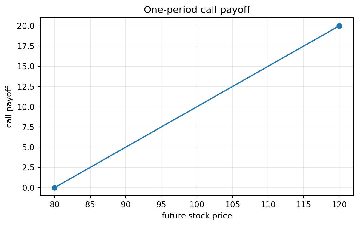
S_0=100,\qquad u=1.2,\qquad d=0.8,\qquad R=1.05.
$$
A European call option with strike $K=100$ has payoffs
$$
X_u=(120-100)^+=20,
\qquad
X_d=(80-100)^+=0.
$$
The risk-neutral up probability is
$$
q=\frac{1.05-0.8}{1.2-0.8}=0.625.
$$
The option price is
$$
C_0=\frac{1}{1.05}(0.625\cdot 20+0.375\cdot 0)=11.9048.
$$
The replicating stock holding is
$$
\Delta=\frac{20-0}{100(1.2-0.8)}=0.5.
$$
The bank-account position is
$$
B=\frac{1.2\cdot 0-0.8\cdot 20}{1.05(1.2-0.8)}=-38.0952.
$$
Thus the call can be replicated by buying $0.5$ shares and borrowing $38.0952$ dollars. The initial cost is
$$
0.5(100)-38.0952=11.9048.
$$
:::
## 3.14 Interactive: Binomial Risk-Neutral Pricing
The following interactive demo changes the binomial parameters and recomputes the risk-neutral probability, call payoff, and no-arbitrage price.
::: {.interactive-card}
### Binomial call-pricing explorer
Use the sliders to observe how the option price depends on the stock price, strike, riskless return, and up/down factors.
<div class="mf-controls">
<label for="ch03-s0">Current stock price $S_0$</label>
<output id="ch03-s0-out">100</output>
<input id="ch03-s0" type="range" min="50" max="150" step="1" value="100">
<label for="ch03-k">Strike $K$</label>
<output id="ch03-k-out">100</output>
<input id="ch03-k" type="range" min="50" max="150" step="1" value="100">
<label for="ch03-r">Gross riskless return $R$</label>
<output id="ch03-r-out">1.05</output>
<input id="ch03-r" type="range" min="0.90" max="1.20" step="0.01" value="1.05">
<label for="ch03-u">Up factor $u$</label>
<output id="ch03-u-out">1.20</output>
<input id="ch03-u" type="range" min="1.01" max="1.80" step="0.01" value="1.20">
<label for="ch03-d">Down factor $d$</label>
<output id="ch03-d-out">0.80</output>
<input id="ch03-d" type="range" min="0.30" max="0.99" step="0.01" value="0.80">
</div>
<div id="ch03-binomial-summary" class="mf-output"></div>
<div id="ch03-binomial-plot" class="plotly-demo"></div>
<script>
(function() {
function getNumber(id) {
return parseFloat(document.getElementById(id).value);
}
function fmt(x) {
return Number.isFinite(x) ? x.toFixed(4) : "not defined";
}
function updateBinomialDemo() {
const S0 = getNumber("ch03-s0");
const K = getNumber("ch03-k");
const R = getNumber("ch03-r");
const u = getNumber("ch03-u");
const d = getNumber("ch03-d");
document.getElementById("ch03-s0-out").value = S0.toFixed(0);
document.getElementById("ch03-k-out").value = K.toFixed(0);
document.getElementById("ch03-r-out").value = R.toFixed(2);
document.getElementById("ch03-u-out").value = u.toFixed(2);
document.getElementById("ch03-d-out").value = d.toFixed(2);
const Su = u * S0;
const Sd = d * S0;
const Xu = Math.max(Su - K, 0);
const Xd = Math.max(Sd - K, 0);
const noArb = (d < R && R < u);
const q = (R - d) / (u - d);
const price = (q * Xu + (1 - q) * Xd) / R;
const delta = (Xu - Xd) / (S0 * (u - d));
const bank = (u * Xd - d * Xu) / (R * (u - d));
const summary = noArb
? `<strong>No-arbitrage condition:</strong> satisfied because d < R < u.<br>
<strong>Risk-neutral up probability:</strong> q = ${fmt(q)}.<br>
<strong>Call price:</strong> C0 = ${fmt(price)}.<br>
<strong>Replicating portfolio:</strong> Delta = ${fmt(delta)}, bank position B = ${fmt(bank)}.`
: `<strong>No-arbitrage condition:</strong> violated because d < R < u is false.<br>
The formula produces q = ${fmt(q)}, which is not a valid probability.`;
document.getElementById("ch03-binomial-summary").innerHTML = summary;
const payoffTrace = {
x: [Sd, Su],
y: [Xd, Xu],
mode: "markers+lines",
name: "call payoff at states",
marker: {size: 12}
};
const stockTrace = {
x: [Sd, Su],
y: [0, 0],
mode: "markers",
name: "future stock states",
marker: {size: 10}
};
const layout = {
title: "One-period call payoff across future states",
xaxis: {title: "Future stock price S1"},
yaxis: {title: "Option payoff"},
margin: {l: 60, r: 25, t: 55, b: 55}
};
Plotly.react("ch03-binomial-plot", [payoffTrace, stockTrace], layout, {responsive: true});
}
["ch03-s0", "ch03-k", "ch03-r", "ch03-u", "ch03-d"].forEach(function(id) {
document.getElementById(id).addEventListener("input", updateBinomialDemo);
});
updateBinomialDemo();
})();
</script>
:::
## 3.15 Complete Markets
A market is complete if every claim can be replicated.
::: {.definition}
### Definition 3.7: Complete market
A finite one-period market is **complete** if every claim $X\in\mathbb R^m$ is attainable. Equivalently,
$$
\operatorname{Col}(A)=\mathbb R^m.
$$
:::
Because $A$ is an $m\times(d+1)$ matrix, completeness is equivalent to
$$
\operatorname{rank}(A)=m.
$$
Thus a complete market must have at least as many linearly independent traded payoff vectors as there are states.
::: {.theorem}
### Theorem 3.4: Completeness and uniqueness of state prices
Assume a finite one-period market satisfies no arbitrage. The market is complete if and only if the state-price vector $q$ satisfying
$$
A^\top q=S_0
$$
is unique.
:::
::: {.proof}
If the market is complete, then $\operatorname{Col}(A)=\mathbb R^m$, so $A$ has rank $m$. Therefore $A^\top$ has rank $m$, and the linear system $A^\top q=S_0$ has at most one solution.
Conversely, if the market is not complete, then $\operatorname{Col}(A)$ is a proper subspace of $\mathbb R^m$. There exists a nonzero vector $z$ orthogonal to every attainable payoff, so
$$
A^\top z=0.
$$
If $q$ is one state-price vector, then $q+\varepsilon z$ also satisfies
$$
A^\top(q+\varepsilon z)=A^\top q=S_0.
$$
For sufficiently small $\varepsilon$, positivity is preserved. Hence the state-price vector is not unique.
:::
Completeness is a mathematical idealization. Real markets are incomplete because not every possible future payoff can be perfectly replicated. However, complete models are valuable because they give unique prices and explicit hedging strategies.
## 3.16 Incomplete Markets and Price Bounds
If a claim is not attainable, no-arbitrage may not determine a unique price. Instead, it gives an interval of admissible prices.
Suppose $q$ ranges over all strictly positive state-price vectors satisfying
$$
A^\top q=S_0.
$$
For a nonattainable claim $X$, any price of the form
$$
\pi_q(X)=q^\top X
$$
is consistent with the traded assets. Therefore no-arbitrage prices are constrained by
$$
\inf_{q>0,\ A^\top q=S_0} q^\top X
\le \pi(X) \le
\sup_{q>0,\ A^\top q=S_0} q^\top X.
$$
With non-strict positivity $q\ge 0$, these become closed super- and sub-replication bounds.
::: {.definition}
### Definition 3.8: No-arbitrage price bounds
The **lower no-arbitrage bound** of a claim $X$ is the largest price below which selling the claim creates arbitrage. The **upper no-arbitrage bound** is the smallest price above which buying the claim creates arbitrage.
In finite-state models, these bounds can be computed by optimizing $q^\top X$ over the state-price polytope.
:::
## 3.17 Worked Incomplete-Market Example
Consider three states and two traded assets: a bank account and a stock. Let
$$
R=1.05,
\qquad
S_0=100,
$$
and
$$
S_1=70,100,140
$$
in states $\omega_1,\omega_2,\omega_3$. A state-price vector $q=(q_1,q_2,q_3)$ must satisfy
$$
q_1+q_2+q_3=\frac{1}{1.05},
$$
and
$$
70q_1+100q_2+140q_3=100.
$$
There are three unknowns and two equations. Hence the state-price vector is not unique. This market is incomplete.
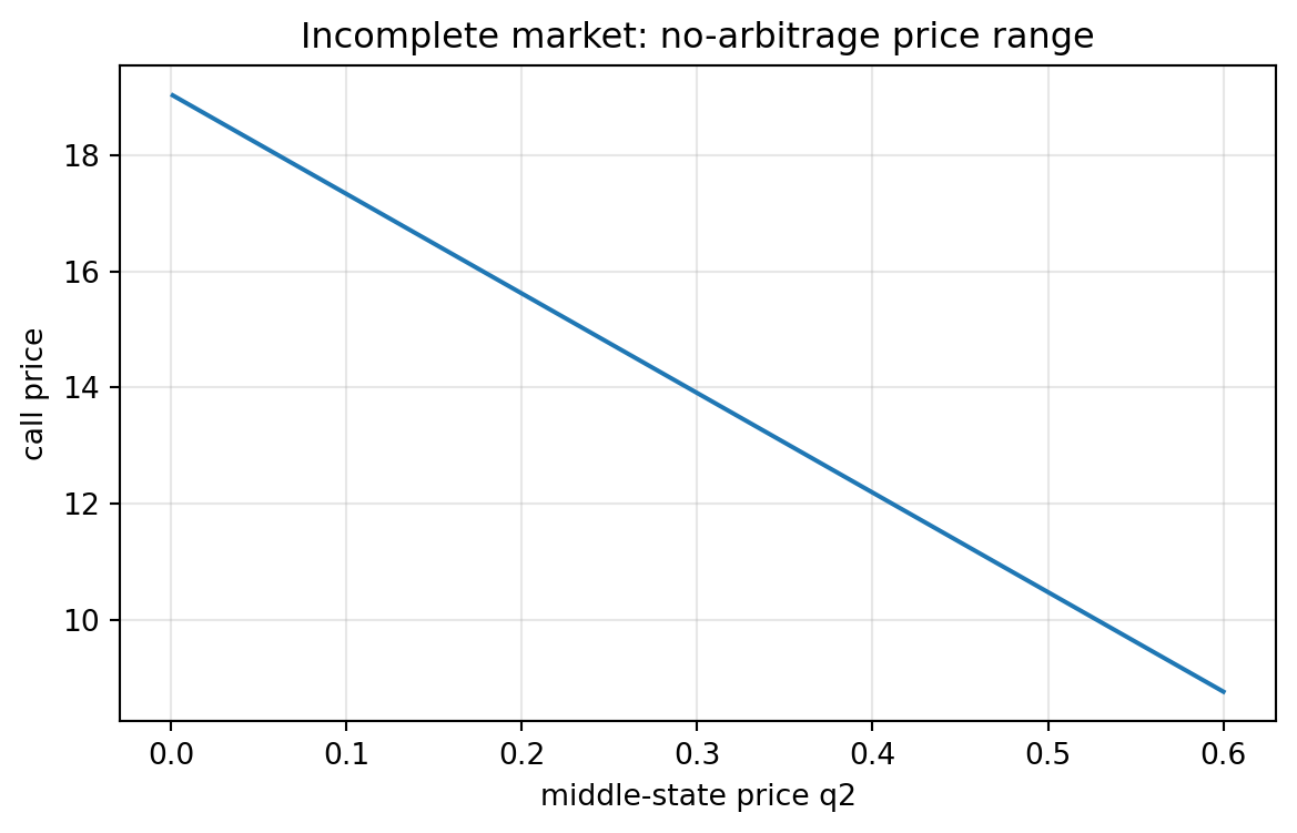
Let $X=(0,0,40)$ be a call payoff with strike $100$. Its possible no-arbitrage prices are
$$
q^\top X=40q_3,
$$
where $q$ ranges over the positive solutions of the two equations. Different choices of state prices give different arbitrage-free call prices.
This example shows why incomplete markets require additional modeling assumptions, utility preferences, calibration choices, or hedging criteria.
## 3.18 Interactive: State-Price Polytope in a Three-State Market
The next demo illustrates the incomplete three-state model above. Changing the free state price $q_2$ moves along the state-price line and changes the price of a nonreplicable call payoff.
::: {.interactive-card}
### Three-state state-price explorer
<div class="mf-controls">
<label for="ch03-q2">Middle-state price $q_2$</label>
<output id="ch03-q2-out">0.300</output>
<input id="ch03-q2" type="range" min="0.001" max="0.60" step="0.001" value="0.300">
</div>
<div id="ch03-stateprice-summary" class="mf-output"></div>
<div id="ch03-stateprice-plot" class="plotly-demo"></div>
<script>
(function() {
function solveQ(q2) {
const R = 1.05;
const sum = 1 / R;
const S0 = 100;
const s1 = 70;
const s2 = 100;
const s3 = 140;
const remainingSum = sum - q2;
const remainingStock = S0 - s2 * q2;
const q3 = (remainingStock - s1 * remainingSum) / (s3 - s1);
const q1 = remainingSum - q3;
return {q1, q2, q3, R};
}
function updateStatePriceDemo() {
const q2 = parseFloat(document.getElementById("ch03-q2").value);
document.getElementById("ch03-q2-out").value = q2.toFixed(3);
const ans = solveQ(q2);
const callPrice = 40 * ans.q3;
const positive = ans.q1 > 0 && ans.q2 > 0 && ans.q3 > 0;
const Q1 = ans.R * ans.q1;
const Q2 = ans.R * ans.q2;
const Q3 = ans.R * ans.q3;
document.getElementById("ch03-stateprice-summary").innerHTML =
`<strong>q = </strong>(${ans.q1.toFixed(4)}, ${ans.q2.toFixed(4)}, ${ans.q3.toFixed(4)}).<br>` +
`<strong>Positive state prices?</strong> ${positive ? "yes" : "no"}.<br>` +
`<strong>Risk-neutral Q = </strong>(${Q1.toFixed(4)}, ${Q2.toFixed(4)}, ${Q3.toFixed(4)}).<br>` +
`<strong>Call payoff X=(0,0,40) price:</strong> ${callPrice.toFixed(4)}.`;
const q2Vals = [];
const callVals = [];
const colors = [];
for (let k = 1; k <= 600; k++) {
const x = k / 1000;
const q = solveQ(x);
q2Vals.push(x);
callVals.push(40 * q.q3);
colors.push((q.q1 > 0 && q.q2 > 0 && q.q3 > 0) ? 1 : 0);
}
const curve = {
x: q2Vals,
y: callVals,
mode: "lines",
name: "call price as q2 varies"
};
const point = {
x: [q2],
y: [callPrice],
mode: "markers",
name: "selected state price",
marker: {size: 12}
};
const layout = {
title: "Incomplete market: a range of no-arbitrage prices",
xaxis: {title: "middle-state price q2"},
yaxis: {title: "price of X=(0,0,40)"},
margin: {l: 60, r: 25, t: 55, b: 55}
};
Plotly.react("ch03-stateprice-plot", [curve, point], layout, {responsive: true});
}
document.getElementById("ch03-q2").addEventListener("input", updateStatePriceDemo);
updateStatePriceDemo();
})();
</script>
:::
## 3.19 Python Example: Binomial Replication
The following Python code implements the replication and risk-neutral pricing formulas for a one-period call.
```{python}
#| label: py-ch03-binomial-replication
#| fig-cap: "One-period call payoff in the binomial model."
import numpy as np
import matplotlib.pyplot as plt

S0 = 100.0
u = 1.20
d = 0.80
R = 1.05
K = 100.0

Su = u * S0
Sd = d * S0
Xu = max(Su - K, 0.0)
Xd = max(Sd - K, 0.0)

q = (R - d) / (u - d)
price_rn = (q * Xu + (1 - q) * Xd) / R

delta = (Xu - Xd) / (S0 * (u - d))
bank = (u * Xd - d * Xu) / (R * (u - d))
price_rep = delta * S0 + bank

print("risk-neutral up probability:", q)
print("risk-neutral price:", price_rn)
print("delta:", delta)
print("bank position:", bank)
print("replication price:", price_rep)

future_stock = np.array([Sd, Su])
future_payoff = np.array([Xd, Xu])

plt.figure(figsize=(7, 4))
plt.plot(future_stock, future_payoff, marker="o")
plt.xlabel("future stock price")
plt.ylabel("call payoff")
plt.title("One-period call payoff")
plt.grid(True, alpha=0.3)
plt.show()
```
The equality of `price_rn` and `price_rep` is not an accident. The first calculation uses the pricing measure; the second uses a trading strategy. In a complete one-period model, they are two views of the same no-arbitrage price.
## 3.20 Python Example: State Prices from a Linear System
The next computation solves
$$
A^\top q=S_0
$$
for a complete two-state model.
```{python}
#| label: py-ch03-state-prices-complete
import numpy as np

S0_stock = 100.0
R = 1.05
u = 1.20
d = 0.80

A = np.array([
    [R, u * S0_stock],
    [R, d * S0_stock]
])
price_vector = np.array([1.0, S0_stock])

q_state = np.linalg.solve(A.T, price_vector)
Q_rn = R * q_state

print("payoff matrix A:")
print(A)
print("state prices q:", q_state)
print("risk-neutral probabilities Q:", Q_rn)
print("sum of state prices:", q_state.sum())
print("1/R:", 1 / R)
print("sum of risk-neutral probabilities:", Q_rn.sum())
```
This calculation emphasizes the normalization:
$$
Q_i=Rq_i.
$$
The state prices sum to the discount factor $1/R$, while the risk-neutral probabilities sum to $1$.
## 3.21 Python Example: Incomplete Market Price Bounds
Now consider the three-state market from Section 3.17. We compute the possible call prices by scanning feasible positive state prices.
```{python}
#| label: py-ch03-incomplete-market-bounds
#| fig-cap: "No-arbitrage price range for a nonreplicable call in an incomplete one-period market."
import numpy as np
import matplotlib.pyplot as plt

R = 1.05
S0 = 100.0
stock_states = np.array([70.0, 100.0, 140.0])
call_payoff = np.maximum(stock_states - 100.0, 0.0)

def state_prices_from_q2(q2):
    # Equations:
    # q1 + q2 + q3 = 1/R
    # 70 q1 + 100 q2 + 140 q3 = S0
    total = 1.0 / R
    remaining_sum = total - q2
    remaining_stock_value = S0 - stock_states[1] * q2
    q3 = (remaining_stock_value - stock_states[0] * remaining_sum) / (stock_states[2] - stock_states[0])
    q1 = remaining_sum - q3
    return np.array([q1, q2, q3])

q2_grid = np.linspace(0.001, 0.60, 600)
feasible_q = []
prices = []

for q2 in q2_grid:
    q = state_prices_from_q2(q2)
    if np.all(q > 0):
        feasible_q.append(q)
        prices.append(q @ call_payoff)

feasible_q = np.array(feasible_q)
prices = np.array(prices)

print("number of feasible grid points:", len(prices))
print("approximate lower price bound:", prices.min())
print("approximate upper price bound:", prices.max())

plt.figure(figsize=(7, 4))
plt.plot(feasible_q[:, 1], prices)
plt.xlabel("middle-state price q2")
plt.ylabel("call price")
plt.title("Incomplete market: no-arbitrage price range")
plt.grid(True, alpha=0.3)
plt.show()
```
Because the claim is not uniquely replicable, no-arbitrage gives an interval of prices rather than one price.
## 3.22 Python Example: Testing Attainability
A claim $X$ is attainable if the linear system
$$
A\theta=X
$$
has a solution. Numerically, we can solve a least-squares problem and check the residual.
```{python}
#| label: py-ch03-attainability-test
import numpy as np

R = 1.05
S0 = 100.0
stock_states = np.array([70.0, 100.0, 140.0])

A = np.column_stack([
    R * np.ones(3),
    stock_states
])

claims = {
    "stock itself": stock_states,
    "bank account": R * np.ones(3),
    "call strike 100": np.maximum(stock_states - 100.0, 0.0),
    "linear payoff 2 + 0.3 S": 2.0 + 0.3 * stock_states
}

for name, X in claims.items():
    theta, residuals, rank, singular_values = np.linalg.lstsq(A, X, rcond=None)
    error = np.linalg.norm(A @ theta - X)
    print(f"{name:20s} | theta = {theta} | residual norm = {error:.6e}")
```
The call payoff is not affine in the stock price across the three states, so it is not attainable with only the bank account and stock. A linear payoff in the stock price is attainable.
## 3.23 AI-Assisted Learning Components
::: {.ai-box}
### AI check 1: Definitions audit
Ask an AI tool:
> In a finite one-period asset-pricing model, explain the difference between a physical probability, a state-price vector, and a risk-neutral probability. Give one example where the physical probability is different from the risk-neutral probability.
Then check whether the answer correctly states that $Q_i=Rq_i$ when the riskless gross return is $R$.
:::
::: {.ai-box}
### AI check 2: Proof critique
Give an AI tool the proof of the law of one price from this chapter and ask:
> Identify every place where the no-arbitrage assumption is used. Could the conclusion fail if arbitrage exists? Construct a small numerical example.
A good answer should produce two portfolios with identical future payoffs but different initial costs.
:::
::: {.ai-box}
### AI check 3: Code audit
Give an AI tool the Python binomial-pricing code and ask:
> Find edge cases where this code may produce misleading output. What conditions should be checked before computing the risk-neutral probability?
The answer should mention the no-arbitrage condition $d<R<u$, the requirement $u\ne d$, and the positivity of $S_0$.
:::
::: {.ai-box}
### AI check 4: Mathematical explanation test
Ask an AI tool to explain why the formula
$$
\pi(X)=\frac{1}{R}\mathbb E^{\mathbb Q}[X]
$$
does not mean that investors are actually risk neutral. Revise the response until it clearly distinguishes a pricing measure from a behavioral assumption.
:::
## 3.24 Common Mistakes
1. **Using physical probabilities for pricing without justification.** Physical probabilities are useful for prediction and risk management, but no-arbitrage pricing uses state prices or risk-neutral probabilities.
2. **Forgetting discounting.** The risk-neutral formula is
$$
\pi(X)=\frac{1}{R}\mathbb E^{\mathbb Q}[X],
$$
not simply $\mathbb E^{\mathbb Q}[X]$.
3. **Assuming every payoff is attainable.** A market is complete only when $\operatorname{rank}(A)=m$.
4. **Ignoring positivity of state prices.** Solving $A^\top q=S_0$ is not enough. For no-arbitrage, state prices must be positive for economically possible states.
5. **Confusing uniqueness with existence.** No-arbitrage gives existence of positive state prices. Completeness gives uniqueness.
6. **Treating the binomial formula as universal.** The formula $q=(R-d)/(u-d)$ is specific to a two-state one-stock model with a bank account.
## 3.25 Exercises
### Conceptual Exercises
1. Explain why a one-period model can be studied using finite-dimensional linear algebra.
2. Define an arbitrage portfolio. Why is a portfolio with high expected return not necessarily an arbitrage?
3. Explain the difference between an attainable claim and a nonattainable claim.
4. State the law of one price and explain why it follows from no-arbitrage.
5. Explain why state prices must be positive in a no-arbitrage model.
6. Explain why the risk-neutral probability is generally not the same as the physical probability.
### Computational Exercises
7. In a one-period binomial model, let
$$
S_0=50,\quad u=1.3,\quad d=0.7,\quad R=1.04.
$$
Compute the risk-neutral up probability.
8. For the model in Exercise 7, price a European call with strike $K=55$.
9. Compute the replicating portfolio for the call in Exercise 8.
10. Verify directly that the future payoff of the replicating portfolio equals the call payoff in both states.
### Linear Algebra Exercises
11. Let
$$
A=\begin{bmatrix}
1.05 & 120\\
1.05 & 80
\end{bmatrix},
\qquad
S_0=\begin{bmatrix}1\\100\end{bmatrix}.
$$
Solve $A^\top q=S_0$ and convert $q$ into a risk-neutral probability vector.
12. Consider a three-state model with bank account payoff $1.05$ and stock payoffs $70,100,140$. Show that the market with only the bank account and stock is incomplete.
13. In Exercise 12, determine whether the payoff $X=(5,10,15)^\top$ is attainable.
14. In Exercise 12, determine whether the payoff $Y=(0,0,40)^\top$ is attainable.
15. Let $A$ be an $m\times(d+1)$ payoff matrix. Prove that the market can be complete only if $d+1\ge m$.
### Proof Exercises
16. Prove that if a strictly positive state-price vector exists, then the market has no arbitrage.
17. Prove that if the market is complete and no-arbitrage holds, then every claim has a unique no-arbitrage price.
18. Prove the binomial no-arbitrage condition $d<R<u$.
19. Derive the binomial replication formulas
$$
\Delta=\frac{X_u-X_d}{S_0(u-d)},
\qquad
B=\frac{uX_d-dX_u}{R(u-d)}.
$$
20. Show algebraically that the replication price equals the risk-neutral expectation price in the binomial model.
### Python Exercises
21. Write a Python function `binomial_price(S0, K, u, d, R)` that returns the call price, risk-neutral probability, delta, and bank position.
22. Modify the function from Exercise 21 so that it raises an error if $d<R<u$ is not satisfied.
23. Write code that accepts a payoff matrix $A$ and price vector $S_0$ and solves for a state-price vector when the system has a unique solution.
24. Write code that checks whether a claim $X$ is attainable by computing the least-squares residual of $A\theta=X$.
25. For a three-state incomplete market, plot the range of no-arbitrage prices for calls with strikes $K=80,100,120$.
### AI-Assisted Exercises
26. Ask an AI tool to explain state prices to a student who knows linear algebra but not finance. Rewrite the explanation in your own words and correct any imprecise statements.
27. Ask an AI tool to generate a one-period arbitrage example. Verify the example numerically. If the example is wrong, repair it.
28. Ask an AI tool to compare replication pricing and risk-neutral pricing. Identify which assumptions are needed for the two methods to agree.
29. Ask an AI tool to write Python code for binomial option pricing. Add no-arbitrage checks and unit tests.
30. Ask an AI tool to explain incomplete markets. Make sure the explanation distinguishes price bounds from unique prices.
## 3.26 Chapter Summary
This chapter developed one-period asset pricing as a finite-dimensional mathematical theory.
The main objects are:
- state space $\Omega=\{\omega_1,\ldots,\omega_m\}$;
- payoff vectors $X\in\mathbb R^m$;
- price vector $S_0$;
- payoff matrix $A$;
- portfolio vector $\theta$;
- attainable claims $X=A\theta$;
- state-price vector $q$ satisfying $A^\top q=S_0$;
- risk-neutral probability $Q_i=Rq_i$.
The main principles are:
$$
\text{no arbitrage} \Longleftrightarrow \text{existence of positive state prices},
$$
and, in a model with a riskless asset,
$$
\pi(X)=\frac{1}{R}\mathbb E^{\mathbb Q}[X]
$$
for attainable claims. Completeness gives uniqueness of the pricing measure and hence unique prices for all claims.
These ideas will be extended in Chapter 4 to multi-period binomial models, where one-period pricing is applied repeatedly through backward induction.