---
title: "Chapter 26. Mean--Variance Portfolio Theory"
---
::: {.chapter-objectives}
## Learning Goals
By the end of this chapter, students should be able to:
- represent portfolio returns as linear combinations of asset returns;
- derive portfolio mean and variance using vectors and covariance matrices;
- explain diversification in terms of covariance geometry;
- prove that the covariance matrix is positive semidefinite;
- formulate Markowitz portfolio selection as a constrained quadratic optimization problem;
- derive the global minimum-variance portfolio;
- derive the efficient frontier using Lagrange multipliers;
- incorporate a risk-free asset and derive the tangency portfolio;
- distinguish population portfolio theory from estimated portfolio theory;
- use Python and AI tools to check formulas, audit optimization code, and critique assumptions.
:::
::: {.hero-box}
Portfolio theory is linear algebra applied to uncertainty. A portfolio is a vector of weights. Expected return is a linear function of the weights, while variance is a quadratic form:
$$
\mu_p=w^\top \mu,
\qquad
\sigma_p^2=w^\top \Sigma w.
$$
The core mathematical problem is to choose the weight vector $w$ so that the portfolio has desirable mean and variance. The financial idea is diversification. The mathematical idea is covariance geometry.
:::
## 26.1 From Single Assets to Portfolios
Suppose there are $n$ risky assets. Let
$$
R=
\begin{bmatrix}
R_1\\
R_2\\
\vdots\\
R_n
\end{bmatrix}
$$
be the random vector of one-period asset returns. A portfolio is described by a vector of weights
$$
w=
\begin{bmatrix}
w_1\\
w_2\\
\vdots\\
w_n
\end{bmatrix}.
$$
The weight $w_i$ is the fraction of initial wealth invested in asset $i$. If all wealth is invested in the listed assets, then
$$
\mathbf 1^\top w=1,
$$
where $\mathbf 1=(1,\ldots,1)^\top$.
The portfolio return is
$$
R_p=w^\top R=\sum_{i=1}^n w_iR_i.
$$
This formula is exact for simple one-period returns when weights are measured at the beginning of the period.
::: {.remark}
## Long positions, short positions, and leverage
If $w_i>0$, the portfolio is long asset $i$. If $w_i<0$, the portfolio is short asset $i$. If $\sum_i |w_i|>1$, the portfolio is leveraged even if $\mathbf 1^\top w=1$.
:::
## 26.2 Mean Vector and Covariance Matrix
Define the mean return vector
$$
\mu=\mathbb E[R]
$$
and the covariance matrix
$$
\Sigma=\operatorname{Cov}(R)
=\mathbb E[(R-\mu)(R-\mu)^\top].
$$
The portfolio mean is
$$
\mathbb E[R_p]
=
\mathbb E[w^\top R]
=
w^\top \mu.
$$
The portfolio variance is
$$
\operatorname{Var}(R_p)
=
\operatorname{Var}(w^\top R)
=
w^\top \Sigma w.
$$
The standard deviation $\sigma_p=\sqrt{w^\top\Sigma w}$ is often called the portfolio volatility.
::: {.definition}
## Mean--variance pair
For a portfolio $w$, its **mean--variance pair** is
$$
\left(w^\top\mu,\; w^\top\Sigma w\right).
$$
A portfolio is called **mean--variance efficient** if no other feasible portfolio has both weakly larger mean and weakly smaller variance, with at least one strict improvement.
:::
## 26.3 Covariance Geometry
For any vector $a\in\mathbb R^n$,
$$
a^\top\Sigma a
=
\operatorname{Var}(a^\top R)
\ge 0.
$$
Therefore $\Sigma$ is positive semidefinite. If no nonzero linear combination of asset returns has zero variance, then $\Sigma$ is positive definite.
::: {.theorem}
## Covariance matrices are positive semidefinite
Let $R$ be a random vector with finite second moments and covariance matrix $\Sigma$. Then
$$
a^\top\Sigma a\ge 0
$$
for every vector $a$. Hence $\Sigma$ is positive semidefinite.
:::
::: {.proof}
For any deterministic vector $a$,
$$
a^\top\Sigma a
=
a^\top\mathbb E[(R-\mu)(R-\mu)^\top]a
=
\mathbb E[a^\top(R-\mu)(R-\mu)^\top a].
$$
Since $a^\top(R-\mu)$ is a scalar,
$$
a^\top\Sigma a
=
\mathbb E[(a^\top(R-\mu))^2]
=
\operatorname{Var}(a^\top R)
\ge 0.
$$
:::
This proof is important because it explains why variance is a quadratic form and why portfolio optimization becomes quadratic optimization.
## 26.4 Diversification in the Two-Asset Case
For two assets, write
$$
\mathbb E[R_1]=\mu_1,
\qquad
\mathbb E[R_2]=\mu_2,
$$
$$
\operatorname{Var}(R_1)=\sigma_1^2,
\qquad
\operatorname{Var}(R_2)=\sigma_2^2,
$$
and
$$
\operatorname{Corr}(R_1,R_2)=\rho.
$$
If $w$ is invested in asset 1 and $1-w$ in asset 2, then
$$
\mu_p(w)=w\mu_1+(1-w)\mu_2,
$$
and
$$
\sigma_p^2(w)
=
w^2\sigma_1^2+(1-w)^2\sigma_2^2
+2w(1-w)\rho\sigma_1\sigma_2.
$$
The covariance term controls diversification. When $\rho<1$, combining assets can reduce risk. When $\rho$ is low or negative, diversification can be strong.
The minimum-variance two-asset weight in asset 1 is obtained by differentiating $\sigma_p^2(w)$:
$$
w^*
=
\frac{\sigma_2^2-\rho\sigma_1\sigma_2}
{\sigma_1^2+\sigma_2^2-2\rho\sigma_1\sigma_2}.
$$
::: {.remark}
## Diversification is not just holding many assets
Diversification depends on covariance. Holding many assets that move together may produce little risk reduction. Holding fewer assets with low correlations may produce larger risk reduction.
:::
## 26.5 Interactive Example: Two-Asset Diversification
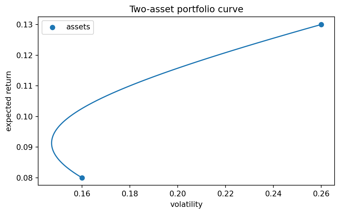
The following interactive example shows how the feasible mean--volatility curve changes with correlation. Lower correlation bends the curve to the left, creating a larger diversification benefit.
::: {.interactive-card}
### Two-asset mean--volatility curve
<div class="mf-control-row">
<label for="ch26-rho">Correlation $\rho$</label>
<input id="ch26-rho" type="range" min="-0.95" max="0.95" step="0.05" value="0.20">
<span id="ch26-rho-val" class="mf-badge">0.20</span>
</div>
<div class="mf-control-row">
<label for="ch26-short">Allow short positions</label>
<input id="ch26-short" type="range" min="0" max="1" step="1" value="0">
<span id="ch26-short-val" class="mf-badge">No</span>
</div>
<div id="ch26-twoasset-demo" class="plotly-demo"></div>
<div id="ch26-twoasset-output" class="mf-output"></div>
:::
<script>
mfPlotlyReady(function() {
var rhoSlider = document.getElementById("ch26-rho");
var shortSlider = document.getElementById("ch26-short");
var rhoVal = document.getElementById("ch26-rho-val");
var shortVal = document.getElementById("ch26-short-val");
var out = document.getElementById("ch26-twoasset-output");
var plotId = "ch26-twoasset-demo";
function draw() {
var rho = parseFloat(rhoSlider.value);
var allowShort = parseInt(shortSlider.value, 10) === 1;
rhoVal.textContent = rho.toFixed(2);
shortVal.textContent = allowShort ? "Yes" : "No";
var mu1 = 0.08, mu2 = 0.13;
var s1 = 0.16, s2 = 0.26;
var wMin = allowShort ? -0.5 : 0.0;
var wMax = allowShort ? 1.5 : 1.0;
var vols = [], means = [], weights = [];
var n = 240;
for (var i = 0; i <= n; i++) {
var w = wMin + (wMax - wMin) * i / n;
var mean = w * mu1 + (1 - w) * mu2;
var variance = w*w*s1*s1 + (1-w)*(1-w)*s2*s2 + 2*w*(1-w)*rho*s1*s2;
vols.push(Math.sqrt(Math.max(variance, 0)));
means.push(mean);
weights.push(w);
}
var denom = s1*s1 + s2*s2 - 2*rho*s1*s2;
var wStar = (s2*s2 - rho*s1*s2) / denom;
var meanStar = wStar * mu1 + (1 - wStar) * mu2;
var varStar = wStar*wStar*s1*s1 + (1-wStar)*(1-wStar)*s2*s2 + 2*wStar*(1-wStar)*rho*s1*s2;
var volStar = Math.sqrt(Math.max(varStar, 0));
var traces = [
{x: vols, y: means, mode: "lines", name: "feasible portfolios", text: weights.map(function(w){return "w1=" + w.toFixed(2);})},
{x: [s1, s2], y: [mu1, mu2], mode: "markers+text", text: ["Asset 1", "Asset 2"], textposition: "top center", name: "individual assets", marker: {size: 10}},
{x: [volStar], y: [meanStar], mode: "markers+text", text: ["GMV"], textposition: "bottom right", name: "minimum variance", marker: {size: 12}}
];
var layout = {
title: "Diversification and correlation",
xaxis: {title: "portfolio volatility"},
yaxis: {title: "expected return", tickformat: ".1%"},
margin: {l: 65, r: 30, t: 55, b: 55},
legend: {orientation: "h"}
};
Plotly.newPlot(plotId, traces, layout, {responsive: true});
out.innerHTML = "Minimum-variance weight in asset 1: $w^*=" + wStar.toFixed(3) + "$. If this weight lies outside $[0,1]$, the unconstrained optimum uses a short or leveraged position.";
}
rhoSlider.addEventListener("input", draw);
shortSlider.addEventListener("input", draw);
draw();
});
</script>
## 26.6 Python Example: Two-Asset Portfolio Curve
```{python}
#| label: ch26-two-asset-curve
#| echo: true
#| warning: false
#| message: false
import numpy as np
import matplotlib.pyplot as plt

mu1, mu2 = 0.08, 0.13
sigma1, sigma2 = 0.16, 0.26
rho = 0.20

weights = np.linspace(0, 1, 201)
means = weights * mu1 + (1 - weights) * mu2
variances = (
    weights**2 * sigma1**2
    + (1 - weights)**2 * sigma2**2
    + 2 * weights * (1 - weights) * rho * sigma1 * sigma2
)
vols = np.sqrt(variances)

w_star = (sigma2**2 - rho * sigma1 * sigma2) / (
    sigma1**2 + sigma2**2 - 2 * rho * sigma1 * sigma2
)
print("Minimum-variance weight in asset 1:", round(w_star, 4))

plt.figure(figsize=(7, 4))
plt.plot(vols, means)
plt.scatter([sigma1, sigma2], [mu1, mu2], label="assets")
plt.xlabel("volatility")
plt.ylabel("expected return")
plt.title("Two-asset portfolio curve")
plt.legend()
plt.show()
```
## 26.7 The Markowitz Optimization Problem
The basic Markowitz problem fixes a target mean return $m$ and minimizes variance:
$$
\begin{aligned}
\min_w \quad & w^\top\Sigma w \\
\text{subject to}\quad & w^\top\mu=m,\\
& w^\top\mathbf 1=1.
\end{aligned}
$$
This is a quadratic optimization problem with linear equality constraints.
The assumptions are strong:
1. the investor cares only about mean and variance;
2. the mean vector $\mu$ is known;
3. the covariance matrix $\Sigma$ is known;
4. trading constraints and transaction costs are ignored;
5. portfolio weights can be chosen continuously.
Despite these limitations, the model is mathematically central because it reveals the geometry of diversification.
## 26.8 Lagrange Multiplier Derivation
Assume $\Sigma$ is positive definite. Let
$$
A=\mathbf 1^\top\Sigma^{-1}\mathbf 1,
\qquad
B=\mathbf 1^\top\Sigma^{-1}\mu,
\qquad
C=\mu^\top\Sigma^{-1}\mu,
$$
and
$$
D=AC-B^2.
$$
The Lagrangian is
$$
L(w,\lambda,\gamma)
=
w^\top\Sigma w
-
\lambda(w^\top\mu-m)
-
\gamma(w^\top\mathbf 1-1).
$$
The first-order condition is
$$
2\Sigma w-\lambda\mu-\gamma\mathbf 1=0.
$$
Thus
$$
w=\frac12\Sigma^{-1}(\lambda\mu+\gamma\mathbf 1).
$$
Solving the two constraints gives the efficient portfolio with target mean $m$:
$$
w(m)
=
\Sigma^{-1}\left[
\frac{A m-B}{D}\mu
+
\frac{C-Bm}{D}\mathbf 1
\right].
$$
The minimum variance at target mean $m$ is
$$
\sigma^2(m)
=
\frac{A m^2-2Bm+C}{D}.
$$
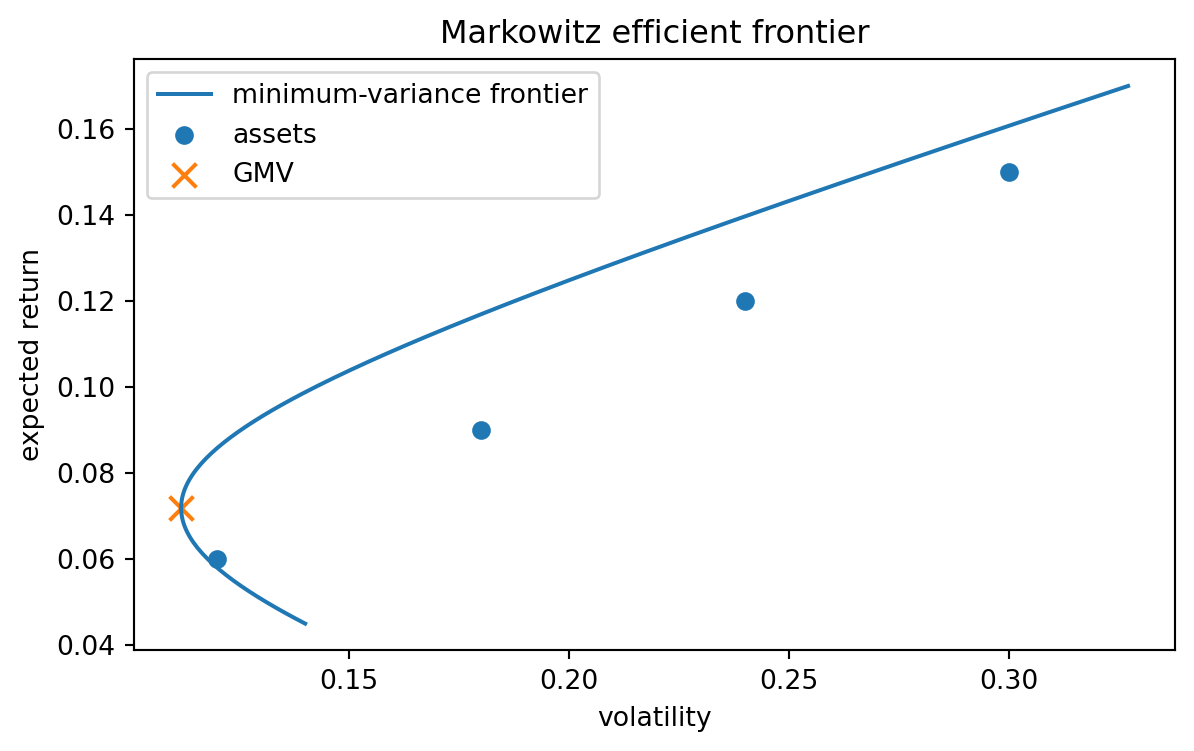
This is the equation of a parabola in mean--variance coordinates. In mean--standard-deviation coordinates, the efficient frontier is the upper branch of a hyperbola.
::: {.theorem}
## Markowitz efficient frontier with equality constraints
Suppose $\Sigma$ is positive definite and $D=AC-B^2>0$. Among all fully invested portfolios with expected return $m$, the unique variance-minimizing portfolio is
$$
w(m)
=
\Sigma^{-1}\left[
\frac{A m-B}{D}\mu
+
\frac{C-Bm}{D}\mathbf 1
\right],
$$
and its variance is
$$
\sigma^2(m)=\frac{A m^2-2Bm+C}{D}.
$$
:::
## 26.9 Global Minimum-Variance Portfolio
The global minimum-variance portfolio solves
$$
\min_w w^\top\Sigma w
\quad\text{subject to}\quad
\mathbf 1^\top w=1.
$$
The solution is
$$
w_{\mathrm{GMV}}
=
\frac{\Sigma^{-1}\mathbf 1}{\mathbf 1^\top\Sigma^{-1}\mathbf 1}
=
\frac{\Sigma^{-1}\mathbf 1}{A}.
$$
Its expected return and variance are
$$
\mu_{\mathrm{GMV}}=\frac{B}{A},
\qquad
\sigma^2_{\mathrm{GMV}}=\frac{1}{A}.
$$
::: {.proof}
The Lagrangian is
$$
L(w,\gamma)=w^\top\Sigma w-\gamma(\mathbf 1^\top w-1).
$$
The first-order condition gives
$$
2\Sigma w=\gamma\mathbf 1,
$$
so $w=c\Sigma^{-1}\mathbf 1$. The constraint $\mathbf 1^\top w=1$ implies
$$
c=\frac{1}{\mathbf 1^\top\Sigma^{-1}\mathbf 1}.
$$
Hence
$$
w_{\mathrm{GMV}}=
rac{\Sigma^{-1}\mathbf 1}{\mathbf 1^\top\Sigma^{-1}\mathbf 1}.
$$
:::
## 26.10 Python Example: Markowitz Frontier by Closed Form
```{python}
#| label: ch26-markowitz-closed-form
#| echo: true
#| warning: false
#| message: false
import numpy as np
import matplotlib.pyplot as plt

mu = np.array([0.06, 0.09, 0.12, 0.15])
vol = np.array([0.12, 0.18, 0.24, 0.30])
corr = np.array([
    [1.00, 0.35, 0.25, 0.15],
    [0.35, 1.00, 0.40, 0.30],
    [0.25, 0.40, 1.00, 0.50],
    [0.15, 0.30, 0.50, 1.00],
])
Sigma = np.outer(vol, vol) * corr
ones = np.ones(len(mu))
Sigma_inv = np.linalg.inv(Sigma)

A = ones @ Sigma_inv @ ones
B = ones @ Sigma_inv @ mu
C = mu @ Sigma_inv @ mu
D = A * C - B**2

w_gmv = Sigma_inv @ ones / A
mu_gmv = w_gmv @ mu
var_gmv = w_gmv @ Sigma @ w_gmv

print("GMV weights:", np.round(w_gmv, 4))
print("GMV expected return:", round(mu_gmv, 4))
print("GMV volatility:", round(np.sqrt(var_gmv), 4))

m_grid = np.linspace(0.045, 0.17, 200)
frontier_var = (A * m_grid**2 - 2 * B * m_grid + C) / D
frontier_vol = np.sqrt(frontier_var)

plt.figure(figsize=(7, 4))
plt.plot(frontier_vol, m_grid, label="minimum-variance frontier")
plt.scatter(vol, mu, label="assets")
plt.scatter([np.sqrt(var_gmv)], [mu_gmv], marker="x", s=80, label="GMV")
plt.xlabel("volatility")
plt.ylabel("expected return")
plt.title("Markowitz efficient frontier")
plt.legend()
plt.show()
```
## 26.11 Interactive Example: Random Portfolios and the Efficient Frontier
The following demo samples random long-only portfolios and compares them with the closed-form unconstrained frontier. The unconstrained frontier may use short positions, so it can lie outside the cloud of long-only portfolios.
::: {.interactive-card}
### Random portfolios versus Markowitz frontier
<div class="mf-control-row">
<label for="ch26-riskaversion">Risk aversion $\alpha$</label>
<input id="ch26-riskaversion" type="range" min="1" max="20" step="1" value="8">
<span id="ch26-riskaversion-val" class="mf-badge">8</span>
</div>
<div class="mf-control-row">
<label for="ch26-corrlevel">Average correlation level</label>
<input id="ch26-corrlevel" type="range" min="0.05" max="0.75" step="0.05" value="0.30">
<span id="ch26-corrlevel-val" class="mf-badge">0.30</span>
</div>
<div id="ch26-frontier-demo" class="plotly-demo"></div>
<div id="ch26-frontier-output" class="mf-output"></div>
:::
<script>
mfPlotlyReady(function() {
var alphaSlider = document.getElementById("ch26-riskaversion");
var corrSlider = document.getElementById("ch26-corrlevel");
var alphaVal = document.getElementById("ch26-riskaversion-val");
var corrVal = document.getElementById("ch26-corrlevel-val");
var out = document.getElementById("ch26-frontier-output");
var plotId = "ch26-frontier-demo";
function matVec(M, v) {
return M.map(function(row) { return row.reduce(function(s, x, i) { return s + x * v[i]; }, 0); });
}
function dot(a, b) {
return a.reduce(function(s, x, i) { return s + x * b[i]; }, 0);
}
function inv4(M) {
var A = M.map(function(row, i) {
var r = row.slice();
for (var j = 0; j < 4; j++) r.push(i === j ? 1 : 0);
return r;
});
for (var i = 0; i < 4; i++) {
var piv = i;
for (var k = i + 1; k < 4; k++) if (Math.abs(A[k][i]) > Math.abs(A[piv][i])) piv = k;
var tmp = A[i]; A[i] = A[piv]; A[piv] = tmp;
var div = A[i][i];
for (var j = 0; j < 8; j++) A[i][j] /= div;
for (var k2 = 0; k2 < 4; k2++) {
if (k2 === i) continue;
var factor = A[k2][i];
for (var j2 = 0; j2 < 8; j2++) A[k2][j2] -= factor * A[i][j2];
}
}
return A.map(function(row) { return row.slice(4); });
}
function lcg(seed) {
var m = 2147483647, a = 48271, state = seed % m;
return function() {
state = (a * state) % m;
return state / m;
};
}
function draw() {
var alpha = parseFloat(alphaSlider.value);
var c = parseFloat(corrSlider.value);
alphaVal.textContent = alpha.toFixed(0);
corrVal.textContent = c.toFixed(2);
var mu = [0.06, 0.09, 0.12, 0.15];
var vol = [0.12, 0.18, 0.24, 0.30];
var ones = [1, 1, 1, 1];
var Sigma = [];
for (var i = 0; i < 4; i++) {
Sigma[i] = [];
for (var j = 0; j < 4; j++) {
var corr = i === j ? 1.0 : c;
Sigma[i][j] = corr * vol[i] * vol[j];
}
}
var Sinv = inv4(Sigma);
var SinvOne = matVec(Sinv, ones);
var SinvMu = matVec(Sinv, mu);
var A = dot(ones, SinvOne);
var B = dot(ones, SinvMu);
var C = dot(mu, SinvMu);
var D = A * C - B * B;
var rng = lcg(26026);
var xs = [], ys = [], utils = [];
for (var s = 0; s < 800; s++) {
var raw = [rng(), rng(), rng(), rng()];
var total = raw.reduce(function(a, b){return a + b;}, 0);
var w = raw.map(function(x){return x / total;});
var mean = dot(w, mu);
var Sw = matVec(Sigma, w);
var variance = dot(w, Sw);
xs.push(Math.sqrt(variance));
ys.push(mean);
utils.push(mean - 0.5 * alpha * variance);
}
var mVals = [], vVals = [];
for (var k = 0; k <= 120; k++) {
var m = 0.04 + 0.13 * k / 120;
var varF = (A * m * m - 2 * B * m + C) / D;
if (varF > 0) {
mVals.push(m);
vVals.push(Math.sqrt(varF));
}
}
var gmvVar = 1 / A;
var gmvMu = B / A;
var traces = [
{x: xs, y: ys, mode: "markers", name: "random long-only portfolios", marker: {size: 5, opacity: 0.45, color: utils, colorscale: "Viridis", showscale: true, colorbar: {title: "utility"}}},
{x: vVals, y: mVals, mode: "lines", name: "unconstrained frontier"},
{x: [Math.sqrt(gmvVar)], y: [gmvMu], mode: "markers+text", text: ["GMV"], textposition: "bottom right", name: "GMV", marker: {size: 12}}
];
var layout = {
title: "Random portfolios and efficient frontier",
xaxis: {title: "volatility"},
yaxis: {title: "expected return", tickformat: ".1%"},
margin: {l: 65, r: 30, t: 55, b: 55},
legend: {orientation: "h"}
};
Plotly.newPlot(plotId, traces, layout, {responsive: true});
out.innerHTML = "The color shows mean--variance utility $U(w)=w^T\\mu - \\frac{\\alpha}{2}w^T\\Sigma w$. Higher correlation reduces the diversification benefit and shifts the portfolio cloud to the right.";
}
alphaSlider.addEventListener("input", draw);
corrSlider.addEventListener("input", draw);
draw();
});
</script>
## 26.12 Mean--Variance Utility
Instead of fixing a target return, an investor may maximize a mean--variance utility function:
$$
U(w)=w^\top\mu-\frac{\alpha}{2}w^\top\Sigma w,
$$
where $\alpha>0$ measures risk aversion. Larger $\alpha$ penalizes variance more strongly.
With only the budget constraint $\mathbf 1^\top w=1$, the first-order condition is
$$
\mu-\alpha\Sigma w-\gamma\mathbf 1=0.
$$
Thus
$$
w=
\frac{1}{\alpha}\Sigma^{-1}(\mu-\gamma\mathbf 1),
$$
where $\gamma$ is chosen so that $\mathbf 1^\top w=1$.
The utility formulation and target-return formulation are two ways to describe the same efficient frontier. Different risk-aversion values choose different points on the frontier.
## 26.13 Risk-Free Asset and the Tangency Portfolio
Suppose investors can borrow or lend at a risk-free return $r_f$. A portfolio that invests fraction $x$ in a risky portfolio $w$ and fraction $1-x$ in the risk-free asset has mean
$$
r_f+x(w^\top\mu-r_f)
$$
and volatility
$$
|x|\sqrt{w^\top\Sigma w}.
$$
The best risky portfolio maximizes the Sharpe ratio
$$
\frac{w^\top\mu-r_f}{\sqrt{w^\top\Sigma w}}
$$
subject to $\mathbf 1^\top w=1$. The solution is the **tangency portfolio**
$$
w_T
=
\frac{\Sigma^{-1}(\mu-r_f\mathbf 1)}
{\mathbf 1^\top\Sigma^{-1}(\mu-r_f\mathbf 1)}.
$$
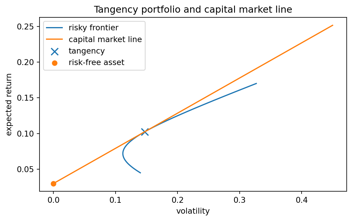
The capital market line is
$$
\mathbb E[R_p]
=
r_f+
rac{\mu_T-r_f}{\sigma_T}\sigma_p.
$$
This line dominates the risky-assets-only frontier when borrowing and lending at $r_f$ are allowed.
## 26.14 Python Example: Tangency Portfolio
```{python}
#| label: ch26-tangency-portfolio
#| echo: true
#| warning: false
#| message: false
rf = 0.03
excess = mu - rf * ones
w_tan = Sigma_inv @ excess
w_tan = w_tan / (ones @ w_tan)

mu_tan = w_tan @ mu
vol_tan = np.sqrt(w_tan @ Sigma @ w_tan)
sharpe_tan = (mu_tan - rf) / vol_tan

print("Tangency weights:", np.round(w_tan, 4))
print("Tangency expected return:", round(mu_tan, 4))
print("Tangency volatility:", round(vol_tan, 4))
print("Tangency Sharpe ratio:", round(sharpe_tan, 4))

sigma_line = np.linspace(0, 0.45, 100)
mean_line = rf + sharpe_tan * sigma_line

plt.figure(figsize=(7, 4))
plt.plot(frontier_vol, m_grid, label="risky frontier")
plt.plot(sigma_line, mean_line, label="capital market line")
plt.scatter([vol_tan], [mu_tan], marker="x", s=80, label="tangency")
plt.scatter([0], [rf], label="risk-free asset")
plt.xlabel("volatility")
plt.ylabel("expected return")
plt.title("Tangency portfolio and capital market line")
plt.legend()
plt.show()
```
## 26.15 Constraints and Real Portfolios
The closed-form formulas above allow short positions and arbitrary leverage. Many real portfolio problems include constraints such as
$$
w_i\ge 0,
\qquad
\sum_i w_i=1,
$$
or box constraints
$$
\ell_i\le w_i\le u_i.
$$
Other realistic constraints include:
- sector exposure constraints;
- turnover constraints;
- transaction costs;
- leverage limits;
- minimum or maximum position sizes;
- benchmark-relative risk constraints.
Once inequality constraints are imposed, the optimization problem is still convex if the covariance matrix is positive semidefinite and the constraints are convex, but closed-form formulas are generally replaced by numerical quadratic programming.
::: {.remark}
## Unconstrained formulas are theory, not always recommendations
A closed-form Markowitz portfolio may contain large long and short positions. This is not a bug in the algebra. It is a sign that the mathematical model lacks practical trading constraints or that the inputs are unstable.
:::
## 26.16 Estimation Risk
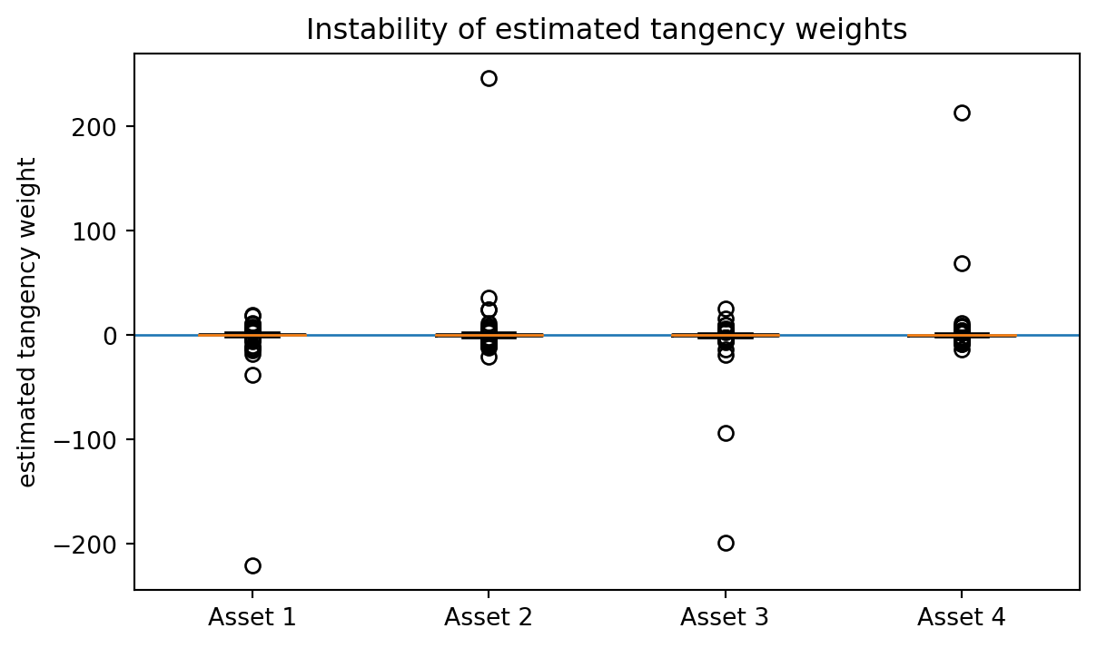
In theory, $\mu$ and $\Sigma$ are known. In practice, they are estimated from data. This creates a major problem: mean estimates are noisy.
If daily returns are independent with daily volatility $\sigma_d$ and $T$ observations, the standard error of the sample mean is approximately
$$
\frac{\sigma_d}{\sqrt{T}}.
$$
Annualized expected returns are especially hard to estimate accurately. As a result, Markowitz portfolios can be extremely sensitive to small changes in $\mu$.
Common responses include:
1. shrinkage of mean estimates;
2. shrinkage of covariance matrices;
3. factor models;
4. robust optimization;
5. constraints on weights;
6. resampling and stability checks.
## 26.17 Python Example: Estimation Instability
```{python}
#| label: ch26-estimation-instability
#| echo: true
#| warning: false
#| message: false
rng = np.random.default_rng(26026)
true_mu = mu
true_Sigma = Sigma
n_assets = len(mu)
T = 252
n_trials = 200
weights = []

for _ in range(n_trials):
    sample = rng.multivariate_normal(true_mu / 252, true_Sigma / 252, size=T)
    mu_hat = sample.mean(axis=0) * 252
    Sigma_hat = np.cov(sample, rowvar=False) * 252
    try:
        inv_hat = np.linalg.inv(Sigma_hat)
        w_hat = inv_hat @ (mu_hat - rf * np.ones(n_assets))
        w_hat = w_hat / np.sum(w_hat)
        weights.append(w_hat)
    except np.linalg.LinAlgError:
        pass

weights = np.array(weights)
print("Mean estimated tangency weights:", np.round(weights.mean(axis=0), 3))
print("Std. dev. of estimated weights:", np.round(weights.std(axis=0), 3))

plt.figure(figsize=(7, 4))
plt.boxplot(weights, labels=[f"Asset {i+1}" for i in range(n_assets)])
plt.axhline(0, linewidth=1)
plt.ylabel("estimated tangency weight")
plt.title("Instability of estimated tangency weights")
plt.show()
```
## 26.18 Factor View of Covariance
For many assets, estimating the full covariance matrix is difficult. A factor model assumes returns have the form
$$
R=\alpha+Bf+\varepsilon,
$$
where:
- $f\in\mathbb R^k$ is a vector of common factors;
- $B$ is the matrix of factor loadings;
- $\varepsilon$ is idiosyncratic noise.
If
$$
\operatorname{Cov}(f)=\Sigma_f,
\qquad
\operatorname{Cov}(\varepsilon)=D,
$$
and factors are uncorrelated with idiosyncratic noise, then
$$
\Sigma=B\Sigma_fB^\top+D.
$$
This representation is useful because $k$ is often much smaller than $n$. It also connects portfolio theory with PCA, regression, and statistical learning.
## 26.19 AI-Assisted Learning Components
AI tools can be useful for portfolio theory, but only if students ask mathematically precise questions and verify the output.
::: {.ai-box}
## AI prompt: formula audit
Ask an AI tool:
> I am deriving the Markowitz efficient frontier. My definitions are $A=1^T\Sigma^{-1}1$, $B=1^T\Sigma^{-1}\mu$, $C=\mu^T\Sigma^{-1}\mu$, and $D=AC-B^2$. Please check the formula for the target-return minimum-variance portfolio and identify all assumptions needed.
Then verify whether the response mentions:
1. positive definiteness or invertibility of $\Sigma$;
2. equality constraints $1^Tw=1$ and $\mu^Tw=m$;
3. the possibility that inequality constraints change the solution;
4. the fact that estimated inputs are not exact model parameters.
:::
::: {.ai-box}
## AI prompt: code review
Ask an AI tool to review portfolio-optimization code for these errors:
- mixing daily and annualized returns;
- using covariance instead of correlation incorrectly;
- forgetting to enforce $\mathbf 1^\top w=1$;
- treating matrix inverse as numerically stable in all cases;
- failing to check whether weights are extreme;
- interpreting an unconstrained solution as automatically practical.
:::
::: {.ai-box}
## AI prompt: model critique
Ask:
> In a graduate mathematical finance course, explain why mean--variance optimization is mathematically elegant but statistically fragile. Separate the issue of optimization geometry from the issue of estimating expected returns.
A strong answer should distinguish the population optimization problem from the empirical estimation problem.
:::
## 26.20 Common Mistakes
1. **Confusing standard deviation and variance.** The Markowitz objective is often written with variance $w^T\Sigma w$, not standard deviation.
2. **Forgetting the budget constraint.** Without $1^Tw=1$, the optimization problem is a different problem.
3. **Ignoring covariance.** Portfolio risk is not the weighted average of individual risks.
4. **Assuming more assets automatically means less risk.** Diversification depends on correlation and covariance.
5. **Treating sample means as reliable.** Expected returns are difficult to estimate.
6. **Using unconstrained weights without interpretation.** Large negative weights represent short positions and leverage.
7. **Mixing time scales.** If $\mu$ is annualized, $\Sigma$ must also be annualized.
## 26.21 Exercises
### Conceptual exercises
1. Explain why expected portfolio return is linear in weights but portfolio variance is quadratic in weights.
2. In the two-asset formula, explain the role of the correlation coefficient $\rho$.
3. Give an example where holding more assets does not significantly reduce portfolio risk.
4. Explain why the covariance matrix must be positive semidefinite.
5. Explain why a portfolio with negative weights is not necessarily invalid mathematically, but may be impractical financially.
### Mathematical exercises
6. Prove that $\operatorname{Var}(w^TR)=w^T\Sigma w$.
7. Derive the two-asset minimum-variance weight
$$
w^*
=
\frac{\sigma_2^2-\rho\sigma_1\sigma_2}
{\sigma_1^2+\sigma_2^2-2\rho\sigma_1\sigma_2}.
$$
8. Derive the global minimum-variance portfolio using Lagrange multipliers.
9. Starting from the target-return Markowitz problem, derive the efficient frontier formula
$$
\sigma^2(m)=\frac{A m^2-2Bm+C}{D}.
$$
10. Prove that the tangency portfolio is proportional to $\Sigma^{-1}(\mu-r_f\mathbf 1)$.
### Computational exercises
11. Generate a random positive definite covariance matrix and compute the global minimum-variance portfolio.
12. Compare the two-asset frontier for $\rho=-0.5$, $0$, $0.5$, and $0.9$.
13. Simulate returns from a multivariate normal model and estimate the efficient frontier from sample data.
14. Study how the tangency portfolio changes when the estimated mean vector is perturbed.
15. Implement a simple long-only portfolio search by sampling random weights and compare it with the unconstrained frontier.
### AI-assisted exercises
16. Ask an AI tool to derive the Markowitz frontier. Identify any missing assumptions or notation errors.
17. Ask an AI tool to explain why covariance matrices are positive semidefinite. Rewrite the explanation as a rigorous proof.
18. Give an AI tool portfolio-optimization Python code with an intentional annualization error. Ask it to find the error, then verify the correction manually.
19. Ask an AI tool to compare Markowitz optimization with factor-model portfolio construction.
20. Ask an AI tool to generate a two-asset diversification example. Check whether its covariance formula is correct.
## 26.22 Chapter Summary
This chapter introduced portfolio theory as a clean application of linear algebra, probability, and optimization. A portfolio is a vector of weights. Its mean is the linear form $w^T\mu$, and its variance is the quadratic form $w^T\Sigma w$. Diversification is governed by covariance, not by the number of assets alone.
The Markowitz model leads to a constrained quadratic optimization problem. With equality constraints and a positive definite covariance matrix, the efficient frontier has a closed-form solution in terms of
$$
A=1^T\Sigma^{-1}1,
\qquad
B=1^T\Sigma^{-1}\mu,
\qquad
C=\mu^T\Sigma^{-1}\mu.
$$
Adding a risk-free asset leads to the tangency portfolio and the capital market line. In practice, however, the model is statistically fragile because expected returns and covariances must be estimated. The mathematics is elegant; the empirical implementation requires caution.