By the end of this chapter, students should be able to:
explain the economic and mathematical assumptions behind the Capital Asset Pricing Model;
derive the capital market line from mean–variance theory with a risk-free asset;
define the market portfolio and explain why it is central in equilibrium pricing;
derive the CAPM equation from the tangency condition for the market portfolio;
interpret beta as a covariance-normalized projection coefficient;
distinguish systematic risk from diversifiable idiosyncratic risk;
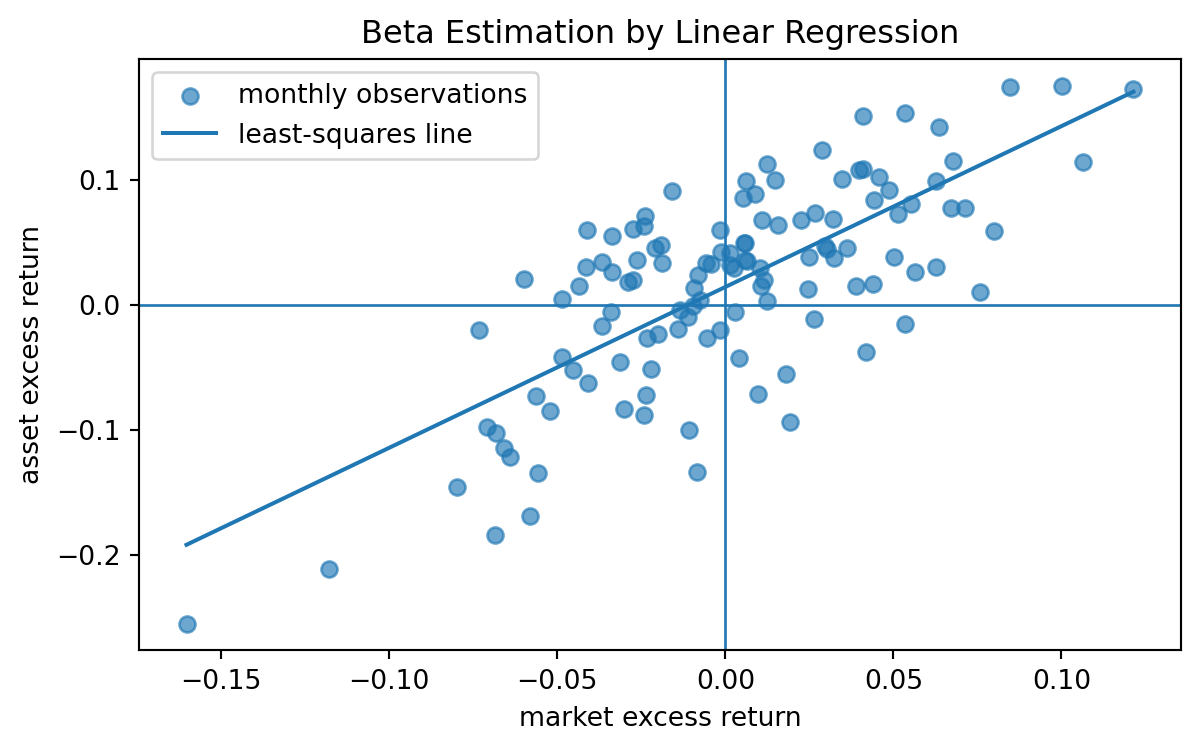
estimate alpha and beta by linear regression;
interpret the security market line and identify mispricing relative to CAPM;
connect CAPM to one-factor models and modern factor investing;
use Python and AI tools to check formulas, audit empirical beta calculations, and critique model assumptions.
CAPM is a bridge between portfolio optimization and asset pricing. Markowitz theory asks: Which portfolio should an investor hold? CAPM asks: If all investors solve a mean–variance problem and markets clear, what expected return should each asset have?
The central conclusion is the security market line:
Only covariance with the market portfolio is priced. Risk that is independent of the market can be diversified away and therefore does not command a risk premium in the model.
30.2 27.1 Why CAPM Follows Portfolio Theory
Chapter 26 studied portfolio choice. Given a vector of expected returns \(\mu\) and a covariance matrix \(\Sigma\), an investor chooses portfolio weights \(w\) to trade off mean and variance:
\[
\mu_p=w^\top\mu,
\qquad
\sigma_p^2=w^\top\Sigma w.
\]
With a risk-free asset available at one-period return \(r_f\), the investor can combine the risk-free asset with a risky portfolio. For a risky portfolio \(p\), define its excess expected return and volatility by
\[
\mu_p-r_f,
\qquad
\sigma_p.
\]
The reward-to-risk ratio of the risky portfolio is the Sharpe ratio
The optimal risky portfolio for a mean–variance investor is the tangency portfolio, the risky portfolio with maximum Sharpe ratio. In equilibrium, if all investors have homogeneous beliefs and can borrow or lend at the same risk-free rate, every investor holds some combination of the risk-free asset and this same tangency portfolio. Since the total supply of risky assets must be held by investors, the tangency portfolio must be the market portfolio.
30.3 Market portfolio
The market portfolio is the value-weighted portfolio of all risky assets in the economy. If asset \(i\) has market value \(V_i\), then its market weight is
\[
w_i^M=\frac{V_i}{\sum_{j=1}^n V_j}.
\]
The return on the market portfolio is
\[
R_M=(w^M)^\top R.
\]
The phrase market portfolio is idealized. In practice, a broad equity index is often used as a proxy, but CAPM itself refers to all risky wealth, not only traded public equities.
30.4 27.2 Model Assumptions
CAPM is mathematically clean because it uses strong assumptions. These assumptions are not minor details; they are exactly what allow an equilibrium pricing relation to be derived from mean–variance optimization.
A standard one-period CAPM uses the following assumptions.
Investors choose portfolios using only mean and variance of one-period returns.
Investors share the same beliefs about \(\mu\) and \(\Sigma\).
A risk-free asset exists and investors can borrow or lend at return \(r_f\).
Assets are infinitely divisible and traded without taxes or transaction costs.
Investors are price takers.
The covariance matrix of risky returns is positive definite on the relevant asset space.
Markets clear: the aggregate demand for risky assets equals the aggregate supply.
Remark (Mathematical role of the assumptions). The assumptions imply that the same tangency portfolio is optimal for all investors. Market clearing then identifies that tangency portfolio with the market portfolio. The CAPM equation is a first-order condition for the market portfolio to be tangent to the efficient frontier.
30.5 27.3 The Capital Market Line
Let \(M\) denote the market portfolio. If an investor invests fraction \(a\) in the market portfolio and fraction \(1-a\) in the risk-free asset, then the portfolio return is
The capital market line is the line in the mean–volatility plane formed by combinations of the risk-free asset and the market portfolio:
\[
\mu_p=r_f+\operatorname{SR}(M)\sigma_p.
\]
It describes efficient portfolios, not individual assets.
This distinction is important. The capital market line is drawn against total volatility \(\sigma_p\). The security market line, derived below, is drawn against beta.
30.7 27.4 Beta as a Projection Coefficient
For an individual risky asset \(i\), define its market beta by
Proof. The market portfolio is the tangency portfolio. Hence \(w^M\) is proportional to \(\Sigma^{-1}(\mu-r_f\mathbf 1)\), which implies \(\mu-r_f\mathbf 1=\lambda\Sigma w^M\). Multiplying by \((w^M)^\top\) gives \(\lambda=(\mu_M-r_f)/\sigma_M^2\). Taking the \(i\)th component gives the result.
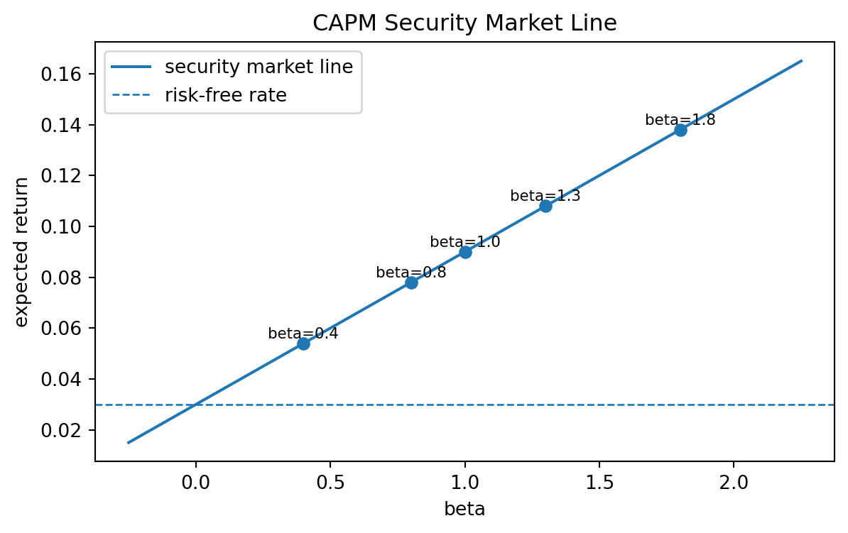
30.11 27.6 Security Market Line
The CAPM equation is a line in the beta–expected-return plane:
\[
\mu_i=r_f+\beta_i(\mu_M-r_f).
\]
30.12 Security market line
The security market line is the graph of expected return as a function of beta:
\[
\mu=r_f+\beta(\mu_M-r_f).
\]
If an asset has expected return above the line, its expected return is high relative to its beta. If an asset has expected return below the line, its expected return is low relative to its beta. In the ideal CAPM equilibrium, all correctly priced assets lie on the line.
30.13 Interactive: security market line
Change the risk-free rate and market risk premium. The security market line moves because CAPM prices beta exposure through the market premium.
The first term is systematic variance. The second term is idiosyncratic variance.
30.15 Systematic risk and idiosyncratic risk
The systematic part of asset \(i\) is the component explained by the market:
\[
\beta_i(R_M-r_f).
\]
The idiosyncratic part is the residual:
\[
\varepsilon_i.
\]
CAPM says the expected excess return compensates investors for systematic risk, not for idiosyncratic risk.
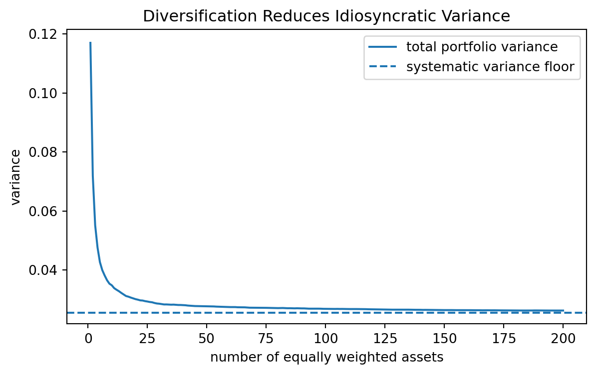
The diversification idea is mathematical. Suppose a portfolio contains many assets whose residuals are weakly correlated. Averaging many residuals reduces idiosyncratic variance, but the common market component remains.
30.16 Interactive: systematic versus idiosyncratic variance
A positive alpha means that the asset’s expected return is above the security market line. A negative alpha means that the expected return is below the line.
30.18 Alpha is not automatically skill
A positive estimated alpha from historical data may come from sampling noise, omitted risk factors, data mining, survivorship bias, transaction costs, or genuine mispricing. The model says what alpha means within the model; statistics is needed to decide whether an estimated alpha is reliable.
30.19 27.9 Portfolio Beta
For a portfolio with weights \(w\), the beta relative to the market is
Now suppose an analyst believes the asset’s expected return is \(13\%\). The CAPM alpha is
\[
\alpha_i
=
0.13-0.114
=
0.016.
\]
This is a \(1.6\%\) expected excess return relative to CAPM. The financial interpretation depends on whether the analyst’s expected return estimate is reliable.
30.24 27.14 Python Example: Diversification of Residual Risk
The following simulation shows why CAPM does not price idiosyncratic risk. We create many assets with the same beta but independent residual shocks. As the number of assets in an equally weighted portfolio grows, residual variance decreases.
This example constructs a small artificial market where expected returns are generated from a market portfolio and a covariance matrix by the CAPM relation
The regression beta is an estimate from finite data. It changes with the sample period, frequency, market proxy, outliers, and changing business conditions.
30.28 27.18 Limitations of CAPM
CAPM is mathematically elegant and historically important, but it is not a complete description of real markets.
Important limitations include:
the true market portfolio is not observable;
expected returns are difficult to estimate;
investors may care about more than mean and variance;
borrowing and lending rates differ;
taxes, transaction costs, constraints, and liquidity matter;
betas can change over time;
empirical returns often show size, value, momentum, profitability, and investment effects;
tail risk and downside risk may matter beyond variance.
These limitations do not make CAPM useless. They explain why CAPM should be read as a baseline model. It teaches the mathematical logic of equilibrium risk pricing and prepares students for multifactor models.
30.29 27.19 AI-Assisted Learning Components
30.30 AI prompt: explain beta as projection
Ask an AI assistant:
Explain why beta equals the slope in the \(L^2\) projection of an asset’s excess return on the market excess return. Use covariance formulas, not only finance intuition.
Because high-volatility assets are riskier, CAPM says they must have higher expected returns.
Ask it to identify the error. A correct answer should say that CAPM prices beta, not total volatility.
30.32 AI prompt: code review for beta estimation
Ask an AI assistant to review code that estimates beta from returns. The review should check:
whether returns or prices are being used;
whether excess returns are used;
whether the market proxy is clearly specified;
whether the covariance and variance use consistent degrees of freedom;
whether alpha uncertainty is reported.
30.33 27.20 Common Mistakes
Confusing CML and SML. The capital market line uses total volatility and applies to efficient portfolios. The security market line uses beta and applies to individual assets and portfolios.
Pricing total variance. CAPM prices systematic risk, not idiosyncratic risk.
Ignoring the market proxy problem. A broad stock index is not the theoretical market portfolio.
Treating estimated beta as fixed. Empirical beta depends on data choices and may change over time.
Interpreting alpha without inference. A nonzero sample alpha may be statistical noise.
Forgetting the risk-free rate. CAPM is naturally written in excess returns.
30.34 27.21 Exercises
30.34.1 Conceptual exercises
Explain why the market portfolio is the tangency portfolio in the CAPM equilibrium.
Distinguish the capital market line from the security market line.
Why does CAPM not reward idiosyncratic risk?
Give an example of an asset with high volatility but low beta.
Explain why the market portfolio is difficult to observe in practice.
30.34.2 Mathematical exercises
Derive the capital market line from a portfolio that invests fraction \(a\) in the market portfolio and \(1-a\) in the risk-free asset.
Prove that portfolio beta satisfies \(\beta_p=w^\top\beta\).
Starting from \(w^M\propto\Sigma^{-1}(\mu-r_f\mathbf 1)\), derive the CAPM equation.
Prove the variance decomposition \[
\operatorname{Var}(R_i)=\beta_i^2\operatorname{Var}(R_M)+\operatorname{Var}(\varepsilon_i)
\] under the condition \(\operatorname{Cov}(\varepsilon_i,R_M)=0\).
Suppose \(\rho_{iM}=0.5\), \(\sigma_i=30\%\), and \(\sigma_M=15\%\). Compute \(\beta_i\).
30.34.3 Computational exercises
Simulate market and asset returns from a one-factor model and estimate beta by regression.
Create a security market line for \(r_f=2\%\) and \(\mu_M=8\%\).
Given betas \((0.6,1.1,1.5)\) and portfolio weights \((0.3,0.4,0.3)\), compute portfolio beta.
Simulate \(100\) assets with independent residuals and show how residual variance decreases in equally weighted portfolios.
Estimate alpha and beta for simulated data and report standard errors.
30.34.4 AI-assisted exercises
Ask an AI assistant to derive CAPM. Identify where it uses the assumption that the market portfolio is tangent.
Ask an AI assistant to explain beta to a statistics student. Require it to use projection and covariance language.
Ask an AI assistant to critique CAPM empirically. Separate mathematical assumptions from empirical failures.
Ask an AI assistant to debug a beta-estimation script that accidentally uses prices instead of returns.
Ask an AI assistant to compare CAPM with a multifactor model. Identify which equation changes.
30.35 27.22 Chapter Summary
CAPM turns mean–variance portfolio theory into an equilibrium asset-pricing model. If all investors hold combinations of the risk-free asset and the market portfolio, then the market portfolio must be the tangency portfolio. The tangency condition implies
Beta is a projection coefficient and measures systematic risk. Idiosyncratic risk can be diversified away and is not priced by CAPM. The model is highly idealized, but it remains a foundational benchmark for understanding risk premia, factor models, and empirical asset pricing.
Source Code
---title: "Chapter 27. Capital Asset Pricing Model"---::: {.chapter-objectives}## Learning GoalsBy the end of this chapter, students should be able to:- explain the economic and mathematical assumptions behind the Capital Asset Pricing Model;- derive the capital market line from mean--variance theory with a risk-free asset;- define the market portfolio and explain why it is central in equilibrium pricing;- derive the CAPM equation from the tangency condition for the market portfolio;- interpret beta as a covariance-normalized projection coefficient;- distinguish systematic risk from diversifiable idiosyncratic risk;- estimate alpha and beta by linear regression;- interpret the security market line and identify mispricing relative to CAPM;- connect CAPM to one-factor models and modern factor investing;- use Python and AI tools to check formulas, audit empirical beta calculations, and critique model assumptions.:::::: {.hero-box}CAPM is a bridge between portfolio optimization and asset pricing. Markowitz theory asks: *Which portfolio should an investor hold?* CAPM asks: *If all investors solve a mean--variance problem and markets clear, what expected return should each asset have?*The central conclusion is the security market line:$$\mathbb E[R_i]-r_f=\beta_i\bigl(\mathbb E[R_M]-r_f\bigr),\qquad\beta_i=\frac{\operatorname{Cov}(R_i,R_M)}{\operatorname{Var}(R_M)}.$$Only covariance with the market portfolio is priced. Risk that is independent of the market can be diversified away and therefore does not command a risk premium in the model.:::## 27.1 Why CAPM Follows Portfolio TheoryChapter 26 studied portfolio choice. Given a vector of expected returns $\mu$ and a covariance matrix $\Sigma$, an investor chooses portfolio weights $w$ to trade off mean and variance:$$\mu_p=w^\top\mu,\qquad\sigma_p^2=w^\top\Sigma w.$$With a risk-free asset available at one-period return $r_f$, the investor can combine the risk-free asset with a risky portfolio. For a risky portfolio $p$, define its excess expected return and volatility by$$\mu_p-r_f,\qquad\sigma_p.$$The reward-to-risk ratio of the risky portfolio is the Sharpe ratio$$\operatorname{SR}(p)=\frac{\mu_p-r_f}{\sigma_p}.$$The optimal risky portfolio for a mean--variance investor is the tangency portfolio, the risky portfolio with maximum Sharpe ratio. In equilibrium, if all investors have homogeneous beliefs and can borrow or lend at the same risk-free rate, every investor holds some combination of the risk-free asset and this same tangency portfolio. Since the total supply of risky assets must be held by investors, the tangency portfolio must be the market portfolio.::: {.definition}## Market portfolioThe **market portfolio** is the value-weighted portfolio of all risky assets in the economy. If asset $i$ has market value $V_i$, then its market weight is$$w_i^M=\frac{V_i}{\sum_{j=1}^n V_j}.$$The return on the market portfolio is$$R_M=(w^M)^\top R.$$:::The phrase *market portfolio* is idealized. In practice, a broad equity index is often used as a proxy, but CAPM itself refers to all risky wealth, not only traded public equities.## 27.2 Model AssumptionsCAPM is mathematically clean because it uses strong assumptions. These assumptions are not minor details; they are exactly what allow an equilibrium pricing relation to be derived from mean--variance optimization.A standard one-period CAPM uses the following assumptions.1. Investors choose portfolios using only mean and variance of one-period returns.2. Investors share the same beliefs about $\mu$ and $\Sigma$.3. A risk-free asset exists and investors can borrow or lend at return $r_f$.4. Assets are infinitely divisible and traded without taxes or transaction costs.5. Investors are price takers.6. The covariance matrix of risky returns is positive definite on the relevant asset space.7. Markets clear: the aggregate demand for risky assets equals the aggregate supply.::: {.remark}## Mathematical role of the assumptionsThe assumptions imply that the same tangency portfolio is optimal for all investors. Market clearing then identifies that tangency portfolio with the market portfolio. The CAPM equation is a first-order condition for the market portfolio to be tangent to the efficient frontier.:::## 27.3 The Capital Market LineLet $M$ denote the market portfolio. If an investor invests fraction $a$ in the market portfolio and fraction $1-a$ in the risk-free asset, then the portfolio return is$$R_a=(1-a)r_f+aR_M.$$Its expected return and standard deviation are$$\mathbb E[R_a]=r_f+a\bigl(\mathbb E[R_M]-r_f\bigr),$$and$$\operatorname{sd}(R_a)=|a|\sigma_M,\qquad\sigma_M=\operatorname{sd}(R_M).$$For $a\ge 0$, eliminating $a$ gives the **capital market line**:$$\mathbb E[R_a]=r_f+ rac{\mathbb E[R_M]-r_f}{\sigma_M}\operatorname{sd}(R_a).$$::: {.definition}## Capital market lineThe **capital market line** is the line in the mean--volatility plane formed by combinations of the risk-free asset and the market portfolio:$$\mu_p=r_f+\operatorname{SR}(M)\sigma_p.$$It describes efficient portfolios, not individual assets.:::This distinction is important. The capital market line is drawn against total volatility $\sigma_p$. The security market line, derived below, is drawn against beta.## 27.4 Beta as a Projection CoefficientFor an individual risky asset $i$, define its market beta by$$\beta_i=\frac{\operatorname{Cov}(R_i,R_M)}{\operatorname{Var}(R_M)}.$$This is the slope coefficient in the best linear prediction of $R_i$ from $R_M$:$$R_i=\alpha_i+\beta_i R_M+\varepsilon_i,\qquad\mathbb E[\varepsilon_i]=0,\qquad\operatorname{Cov}(\varepsilon_i,R_M)=0.$$Thus beta is not just a finance ratio. It is an $L^2$ projection coefficient.::: {.definition}## BetaThe **beta** of asset $i$ relative to the market portfolio is$$\beta_i=\frac{\operatorname{Cov}(R_i,R_M)}{\operatorname{Var}(R_M)}.$$It measures the sensitivity of the asset's return to market movements.:::Using correlation $\rho_{iM}$, beta can also be written as$$\beta_i=\rho_{iM}\frac{\sigma_i}{\sigma_M}.$$An asset can have high volatility and low beta if much of its volatility is idiosyncratic. CAPM prices beta, not total volatility.## 27.5 Deriving the CAPM EquationLet $R=(R_1,\ldots,R_n)^\top$ be the vector of risky asset returns. Let$$\mu=\mathbb E[R],\qquad\Sigma=\operatorname{Cov}(R).$$Let $w^M$ be the market portfolio, so$$R_M=(w^M)^\top R,\qquad\mu_M=(w^M)^\top\mu,\qquad\sigma_M^2=(w^M)^\top\Sigma w^M.$$The market portfolio is the tangency portfolio. Therefore it solves the maximum Sharpe-ratio problem$$\max_w \frac{w^\top\mu-r_f}{\sqrt{w^\top\Sigma w}}\quad \text{subject to} \quad\mathbf 1^\top w=1.$$Equivalently, the tangency portfolio is proportional to$$\Sigma^{-1}(\mu-r_f\mathbf 1).$$Therefore there exists a scalar $c>0$ such that$$w^M=c\Sigma^{-1}(\mu-r_f\mathbf 1).$$Multiplying both sides by $\Sigma$ gives$$\mu-r_f\mathbf 1=\lambda \Sigma w^M$$for some scalar $\lambda>0$. To identify $\lambda$, multiply by $(w^M)^\top$:$$(w^M)^\top(\mu-r_f\mathbf 1)=\lambda (w^M)^\top\Sigma w^M.$$Since $(w^M)^\top\mathbf 1=1$, this becomes$$\mu_M-r_f=\lambda \sigma_M^2.$$Thus$$\lambda=\frac{\mu_M-r_f}{\sigma_M^2}.$$The $i$th component of $\mu-r_f\mathbf 1=\lambda\Sigma w^M$ is$$\mu_i-r_f=\frac{\mu_M-r_f}{\sigma_M^2}(\Sigma w^M)_i.$$But$$(\Sigma w^M)_i=\operatorname{Cov}(R_i,R_M).$$Therefore$$\mu_i-r_f=\frac{\operatorname{Cov}(R_i,R_M)}{\operatorname{Var}(R_M)}(\mu_M-r_f)=\beta_i(\mu_M-r_f).$$This is the CAPM equation.::: {.theorem}## Capital Asset Pricing ModelUnder the one-period CAPM assumptions, every risky asset satisfies$$\mathbb E[R_i]-r_f=\beta_i\bigl(\mathbb E[R_M]-r_f\bigr),$$where$$\beta_i=\frac{\operatorname{Cov}(R_i,R_M)}{\operatorname{Var}(R_M)}.$$:::::: {.proof}The market portfolio is the tangency portfolio. Hence $w^M$ is proportional to $\Sigma^{-1}(\mu-r_f\mathbf 1)$, which implies $\mu-r_f\mathbf 1=\lambda\Sigma w^M$. Multiplying by $(w^M)^\top$ gives $\lambda=(\mu_M-r_f)/\sigma_M^2$. Taking the $i$th component gives the result.:::## 27.6 Security Market LineThe CAPM equation is a line in the beta--expected-return plane:$$\mu_i=r_f+\beta_i(\mu_M-r_f).$$::: {.definition}## Security market lineThe **security market line** is the graph of expected return as a function of beta:$$\mu=r_f+\beta(\mu_M-r_f).$$:::If an asset has expected return above the line, its expected return is high relative to its beta. If an asset has expected return below the line, its expected return is low relative to its beta. In the ideal CAPM equilibrium, all correctly priced assets lie on the line.::: {.interactive-card}## Interactive: security market lineChange the risk-free rate and market risk premium. The security market line moves because CAPM prices beta exposure through the market premium.<div class="mf-control-row"><label for="ch27-rf">Risk-free rate $r_f$</label><input id="ch27-rf" type="range" min="0" max="0.08" step="0.005" value="0.03"><span id="ch27-rf-value" class="mf-badge">3.0%</span></div><div class="mf-control-row"><label for="ch27-premium">Market premium $\mu_M-r_f$</label><input id="ch27-premium" type="range" min="0.01" max="0.12" step="0.005" value="0.06"><span id="ch27-premium-value" class="mf-badge">6.0%</span></div><div id="ch27-sml-demo" class="plotly-demo"></div><div id="ch27-sml-output" class="mf-output"></div><script>(function() {functiondraw() {var rfInput =document.getElementById("ch27-rf");var premiumInput =document.getElementById("ch27-premium");var rfBadge =document.getElementById("ch27-rf-value");var premiumBadge =document.getElementById("ch27-premium-value");var out =document.getElementById("ch27-sml-output");var el =document.getElementById("ch27-sml-demo");if (!rfInput ||!premiumInput ||!el ||typeof Plotly ==="undefined") return;var rf =parseFloat(rfInput.value);var premium =parseFloat(premiumInput.value); rfBadge.textContent= (100* rf).toFixed(1) +"%"; premiumBadge.textContent= (100* premium).toFixed(1) +"%";var betas = [];var returns = [];for (var i =0; i <=80; i++) {var b =-0.25+ i * (2.5/80); betas.push(b); returns.push(rf + b * premium); }var assetBetas = [0.4,0.8,1.0,1.3,1.8];var assetReturns = assetBetas.map(function(b) { return rf + b * premium; });var names = ["Defensive","Low beta","Market","Cyclical","High beta"]; Plotly.newPlot(el, [ {x: betas,y: returns,mode:"lines",name:"Security market line",hovertemplate:"beta=%{x:.2f}<br>expected return=%{y:.2%}<extra></extra>" }, {x: assetBetas,y: assetReturns,text: names,mode:"markers+text",textposition:"top center",name:"Assets on CAPM line",hovertemplate:"%{text}<br>beta=%{x:.2f}<br>expected return=%{y:.2%}<extra></extra>" } ], {title:"CAPM Security Market Line",xaxis: {title:"beta",zeroline:true},yaxis: {title:"expected return",tickformat:".0%"},margin: {l:65,r:25,t:55,b:55},showlegend:true }, {responsive:true}); out.innerHTML="At beta 1, expected return equals the market expected return: "+ (100* (rf + premium)).toFixed(2) +"%. The slope of the line is the market risk premium."; }if (window.mfPlotlyReady) window.mfPlotlyReady(draw);document.addEventListener("input",function(e) {if (e.target&& (e.target.id==="ch27-rf"|| e.target.id==="ch27-premium")) draw(); });})();</script>:::## 27.7 Systematic and Idiosyncratic RiskThe beta projection writes$$R_i-r_f=\alpha_i+\beta_i(R_M-r_f)+\varepsilon_i,\qquad\operatorname{Cov}(\varepsilon_i,R_M)=0.$$In CAPM equilibrium, $\alpha_i=0$ in expectation. The variance decomposes as$$\operatorname{Var}(R_i)=\beta_i^2\operatorname{Var}(R_M)+\operatorname{Var}(\varepsilon_i).$$The first term is **systematic variance**. The second term is **idiosyncratic variance**.::: {.definition}## Systematic risk and idiosyncratic riskThe systematic part of asset $i$ is the component explained by the market:$$\beta_i(R_M-r_f).$$The idiosyncratic part is the residual:$$\varepsilon_i.$$CAPM says the expected excess return compensates investors for systematic risk, not for idiosyncratic risk.:::The diversification idea is mathematical. Suppose a portfolio contains many assets whose residuals are weakly correlated. Averaging many residuals reduces idiosyncratic variance, but the common market component remains.::: {.interactive-card}## Interactive: systematic versus idiosyncratic varianceThis demo shows the decomposition$$\sigma_i^2=\beta_i^2\sigma_M^2+\sigma_{\varepsilon,i}^2.$$<div class="mf-control-row"><label for="ch27-beta">Beta $\beta_i$</label><input id="ch27-beta" type="range" min="0" max="2" step="0.05" value="1.2"><span id="ch27-beta-value" class="mf-badge">1.20</span></div><div class="mf-control-row"><label for="ch27-sigmam">Market volatility $\sigma_M$</label><input id="ch27-sigmam" type="range" min="0.05" max="0.35" step="0.01" value="0.18"><span id="ch27-sigmam-value" class="mf-badge">18%</span></div><div class="mf-control-row"><label for="ch27-sigmaeps">Residual volatility $\sigma_\varepsilon$</label><input id="ch27-sigmaeps" type="range" min="0" max="0.45" step="0.01" value="0.22"><span id="ch27-sigmaeps-value" class="mf-badge">22%</span></div><div id="ch27-risk-demo" class="plotly-demo"></div><div id="ch27-risk-output" class="mf-output"></div><script>(function() {functiondraw() {var beta =parseFloat(document.getElementById("ch27-beta").value);var sigmaM =parseFloat(document.getElementById("ch27-sigmam").value);var sigmaE =parseFloat(document.getElementById("ch27-sigmaeps").value);document.getElementById("ch27-beta-value").textContent= beta.toFixed(2);document.getElementById("ch27-sigmam-value").textContent= (100* sigmaM).toFixed(0) +"%";document.getElementById("ch27-sigmaeps-value").textContent= (100* sigmaE).toFixed(0) +"%";var systematic = beta * beta * sigmaM * sigmaM;var idiosyncratic = sigmaE * sigmaE;var total = systematic + idiosyncratic;var totalVol =Math.sqrt(total);var el =document.getElementById("ch27-risk-demo");if (!el ||typeof Plotly ==="undefined") return; Plotly.newPlot(el, [ {x: ["Systematic","Idiosyncratic","Total"],y: [systematic, idiosyncratic, total],type:"bar",name:"variance",hovertemplate:"%{x}<br>variance=%{y:.4f}<extra></extra>" } ], {title:"Variance Decomposition in a One-Factor Model",yaxis: {title:"variance"},margin: {l:65,r:25,t:55,b:55} }, {responsive:true});document.getElementById("ch27-risk-output").innerHTML="Total volatility is "+ (100* totalVol).toFixed(2) +"%. CAPM prices the beta exposure, not the residual volatility."; }if (window.mfPlotlyReady) window.mfPlotlyReady(draw);document.addEventListener("input",function(e) {if (e.target&& ["ch27-beta","ch27-sigmam","ch27-sigmaeps"].indexOf(e.target.id) >=0) draw(); });})();</script>:::## 27.8 Alpha and Mispricing Relative to CAPMIn empirical finance, one often writes$$R_i-r_f=\alpha_i+\beta_i(R_M-r_f)+\varepsilon_i.$$Taking expectations gives$$\mathbb E[R_i]-r_f=\alpha_i+\beta_i(\mathbb E[R_M]-r_f).$$CAPM predicts$$\alpha_i=0.$$A positive alpha means that the asset's expected return is above the security market line. A negative alpha means that the expected return is below the line.::: {.warning}## Alpha is not automatically skillA positive estimated alpha from historical data may come from sampling noise, omitted risk factors, data mining, survivorship bias, transaction costs, or genuine mispricing. The model says what alpha means within the model; statistics is needed to decide whether an estimated alpha is reliable.:::## 27.9 Portfolio BetaFor a portfolio with weights $w$, the beta relative to the market is$$\beta_p=\frac{\operatorname{Cov}(R_p,R_M)}{\operatorname{Var}(R_M)}.$$Since $R_p=w^\top R$,$$\operatorname{Cov}(R_p,R_M)=\operatorname{Cov}\left(\sum_{i=1}^n w_iR_i,R_M\right)=\sum_{i=1}^n w_i\operatorname{Cov}(R_i,R_M).$$Therefore$$\beta_p=\sum_{i=1}^n w_i\beta_i=w^\top\beta.$$Portfolio beta is a weighted average of asset betas.If every asset satisfies CAPM, then any portfolio also satisfies CAPM:$$\mathbb E[R_p]-r_f=\beta_p(\mathbb E[R_M]-r_f).$$## 27.10 Worked ExampleSuppose the risk-free rate is $r_f=3\%$ and the market expected return is $\mu_M=9\%$. An asset has market beta $\beta_i=1.4$. CAPM gives$$\mathbb E[R_i]=r_f+\beta_i(\mu_M-r_f)=0.03+1.4(0.09-0.03)=0.114.$$The asset's CAPM expected return is $11.4\%$.Now suppose an analyst believes the asset's expected return is $13\%$. The CAPM alpha is$$\alpha_i=0.13-0.114=0.016.$$This is a $1.6\%$ expected excess return relative to CAPM. The financial interpretation depends on whether the analyst's expected return estimate is reliable.## 27.11 Python Example: Security Market Line```{python}#| label: py-ch27-security-market-line#| fig-width: 7#| fig-height: 4import numpy as npimport matplotlib.pyplot as pltr_f =0.03mu_M =0.09market_premium = mu_M - r_fbetas = np.linspace(-0.25, 2.25, 200)expected_returns = r_f + betas * market_premiumasset_betas = np.array([0.4, 0.8, 1.0, 1.3, 1.8])asset_returns = r_f + asset_betas * market_premiumplt.figure(figsize=(7, 4))plt.plot(betas, expected_returns, label="security market line")plt.scatter(asset_betas, asset_returns, zorder=3)for b, m inzip(asset_betas, asset_returns): plt.text(b, m +0.002, f"beta={b:.1f}", ha="center", fontsize=8)plt.axhline(r_f, linestyle="--", linewidth=1, label="risk-free rate")plt.xlabel("beta")plt.ylabel("expected return")plt.title("CAPM Security Market Line")plt.legend()plt.show()```## 27.12 Python Example: Estimating Beta by RegressionSuppose we observe monthly excess returns for an asset and for the market. The regression model is$$R_{i,t}-r_{f,t}=\alpha_i+\beta_i(R_{M,t}-r_{f,t})+\varepsilon_{i,t}.$$The least-squares estimate of beta is$$\widehat\beta_i=\frac{\sum_{t=1}^T (x_t-\bar x)(y_t-\bar y)}{\sum_{t=1}^T (x_t-\bar x)^2},$$where $x_t=R_{M,t}-r_{f,t}$ and $y_t=R_{i,t}-r_{f,t}$.```{python}#| label: py-ch27-beta-regression#| fig-width: 7#| fig-height: 4import numpy as npimport matplotlib.pyplot as pltrng = np.random.default_rng(7243)T =120true_alpha =0.001true_beta =1.35sigma_m =0.045sigma_eps =0.055market_excess = rng.normal(0.006, sigma_m, size=T)epsilon = rng.normal(0.0, sigma_eps, size=T)asset_excess = true_alpha + true_beta * market_excess + epsilonx = market_excessy = asset_excessbeta_hat = np.cov(x, y, ddof=1)[0, 1] / np.var(x, ddof=1)alpha_hat = y.mean() - beta_hat * x.mean()print(f"Estimated alpha: {alpha_hat:.5f}")print(f"Estimated beta: {beta_hat:.3f}")x_grid = np.linspace(x.min(), x.max(), 100)y_grid = alpha_hat + beta_hat * x_gridplt.figure(figsize=(7, 4))plt.scatter(x, y, alpha=0.65, label="monthly observations")plt.plot(x_grid, y_grid, label="least-squares line")plt.axhline(0, linewidth=1)plt.axvline(0, linewidth=1)plt.xlabel("market excess return")plt.ylabel("asset excess return")plt.title("Beta Estimation by Linear Regression")plt.legend()plt.show()```## 27.13 Python Example: Systematic and Idiosyncratic Risk```{python}#| label: py-ch27-risk-decompositionimport numpy as npbeta =1.25sigma_M =0.18sigma_eps =0.20systematic_variance = beta**2* sigma_M**2idiosyncratic_variance = sigma_eps**2total_variance = systematic_variance + idiosyncratic_variancetotal_volatility = np.sqrt(total_variance)print(f"Systematic variance: {systematic_variance:.4f}")print(f"Idiosyncratic variance: {idiosyncratic_variance:.4f}")print(f"Total volatility: {total_volatility:.2%}")print(f"Systematic share: {systematic_variance / total_variance:.2%}")```## 27.14 Python Example: Diversification of Residual RiskThe following simulation shows why CAPM does not price idiosyncratic risk. We create many assets with the same beta but independent residual shocks. As the number of assets in an equally weighted portfolio grows, residual variance decreases.```{python}#| label: py-ch27-diversification-residual-risk#| fig-width: 7#| fig-height: 4import numpy as npimport matplotlib.pyplot as pltrng = np.random.default_rng(5110)T =5000n_assets =200beta =1.0sigma_m =0.16sigma_eps =0.30market = rng.normal(0.0, sigma_m, size=T)residuals = rng.normal(0.0, sigma_eps, size=(T, n_assets))returns = beta * market[:, None] + residualsportfolio_sizes = np.arange(1, n_assets +1)portfolio_variances = []for k in portfolio_sizes: weights = np.ones(k) / k portfolio_return = returns[:, :k] @ weights portfolio_variances.append(np.var(portfolio_return, ddof=1))portfolio_variances = np.array(portfolio_variances)systematic_variance = beta**2* sigma_m**2plt.figure(figsize=(7, 4))plt.plot(portfolio_sizes, portfolio_variances, label="total portfolio variance")plt.axhline(systematic_variance, linestyle="--", label="systematic variance floor")plt.xlabel("number of equally weighted assets")plt.ylabel("variance")plt.title("Diversification Reduces Idiosyncratic Variance")plt.legend()plt.show()```## 27.15 Python Example: Tangency Portfolio Implies CAPMThis example constructs a small artificial market where expected returns are generated from a market portfolio and a covariance matrix by the CAPM relation$$\mu-r_f\mathbf 1=\frac{\mu_M-r_f}{\sigma_M^2}\Sigma w^M.$$Then the tangency portfolio computed from $\Sigma^{-1}(\mu-r_f\mathbf 1)$ matches the market portfolio.```{python}#| label: py-ch27-tangency-implies-capmimport numpy as npSigma = np.array([ [0.0400, 0.0180, 0.0120], [0.0180, 0.0625, 0.0200], [0.0120, 0.0200, 0.0900]])w_M = np.array([0.50, 0.30, 0.20])r_f =0.03mu_M =0.09sigma_M2 = w_M @ Sigma @ w_Mmu = r_f * np.ones(3) + ((mu_M - r_f) / sigma_M2) * (Sigma @ w_M)excess = mu - r_fw_tan_raw = np.linalg.solve(Sigma, excess)w_tan = w_tan_raw / w_tan_raw.sum()betas = (Sigma @ w_M) / sigma_M2capm_mu = r_f + betas * (mu_M - r_f)print("Expected returns:", np.round(mu, 4))print("Betas:", np.round(betas, 4))print("CAPM returns:", np.round(capm_mu, 4))print("Tangency weights:", np.round(w_tan, 4))print("Market weights: ", w_M)```## 27.16 Python Example: Testing Alpha CarefullyA single estimated alpha is not enough. We should ask whether it is statistically distinguishable from zero.```{python}#| label: py-ch27-alpha-t-statisticimport numpy as nprng = np.random.default_rng(7339)T =180true_alpha =0.0005true_beta =1.1sigma_m =0.04sigma_eps =0.06x = rng.normal(0.005, sigma_m, size=T)y = true_alpha + true_beta * x + rng.normal(0.0, sigma_eps, size=T)X = np.column_stack([np.ones(T), x])alpha_hat, beta_hat = np.linalg.lstsq(X, y, rcond=None)[0]resid = y - X @ np.array([alpha_hat, beta_hat])s2 = resid @ resid / (T -2)var_coef = s2 * np.linalg.inv(X.T @ X)se_alpha = np.sqrt(var_coef[0, 0])t_alpha = alpha_hat / se_alphaprint(f"alpha_hat = {alpha_hat:.5f}")print(f"beta_hat = {beta_hat:.3f}")print(f"SE(alpha) = {se_alpha:.5f}")print(f"t(alpha) = {t_alpha:.3f}")```The t-statistic is a reminder that empirical asset pricing is both financial modeling and statistical inference.## 27.17 Relation to Single-Index ModelsCAPM is often taught together with the single-index model$$R_i-r_f=\alpha_i+\beta_i(R_M-r_f)+\varepsilon_i.$$This is a statistical model of returns. CAPM adds an equilibrium pricing restriction:$$\alpha_i=0.$$Thus the single-index model is a regression representation, while CAPM is an economic model that predicts the intercept.::: {.remark}## Regression beta versus true betaThe population beta is$$\beta_i=\frac{\operatorname{Cov}(R_i,R_M)}{\operatorname{Var}(R_M)}.$$The regression beta is an estimate from finite data. It changes with the sample period, frequency, market proxy, outliers, and changing business conditions.:::## 27.18 Limitations of CAPMCAPM is mathematically elegant and historically important, but it is not a complete description of real markets.Important limitations include:- the true market portfolio is not observable;- expected returns are difficult to estimate;- investors may care about more than mean and variance;- borrowing and lending rates differ;- taxes, transaction costs, constraints, and liquidity matter;- betas can change over time;- empirical returns often show size, value, momentum, profitability, and investment effects;- tail risk and downside risk may matter beyond variance.These limitations do not make CAPM useless. They explain why CAPM should be read as a baseline model. It teaches the mathematical logic of equilibrium risk pricing and prepares students for multifactor models.## 27.19 AI-Assisted Learning Components::: {.ai-box}## AI prompt: explain beta as projectionAsk an AI assistant:> Explain why beta equals the slope in the $L^2$ projection of an asset's excess return on the market excess return. Use covariance formulas, not only finance intuition.Then check whether the response explicitly proves$$\beta_i=\frac{\operatorname{Cov}(R_i,R_M)}{\operatorname{Var}(R_M)}.$$:::::: {.ai-box}## AI prompt: audit a CAPM derivationGive an AI assistant the following claim:> Because high-volatility assets are riskier, CAPM says they must have higher expected returns.Ask it to identify the error. A correct answer should say that CAPM prices beta, not total volatility.:::::: {.ai-box}## AI prompt: code review for beta estimationAsk an AI assistant to review code that estimates beta from returns. The review should check:1. whether returns or prices are being used;2. whether excess returns are used;3. whether the market proxy is clearly specified;4. whether the covariance and variance use consistent degrees of freedom;5. whether alpha uncertainty is reported.:::## 27.20 Common Mistakes1. **Confusing CML and SML.** The capital market line uses total volatility and applies to efficient portfolios. The security market line uses beta and applies to individual assets and portfolios.2. **Pricing total variance.** CAPM prices systematic risk, not idiosyncratic risk.3. **Ignoring the market proxy problem.** A broad stock index is not the theoretical market portfolio.4. **Treating estimated beta as fixed.** Empirical beta depends on data choices and may change over time.5. **Interpreting alpha without inference.** A nonzero sample alpha may be statistical noise.6. **Forgetting the risk-free rate.** CAPM is naturally written in excess returns.## 27.21 Exercises### Conceptual exercises1. Explain why the market portfolio is the tangency portfolio in the CAPM equilibrium.2. Distinguish the capital market line from the security market line.3. Why does CAPM not reward idiosyncratic risk?4. Give an example of an asset with high volatility but low beta.5. Explain why the market portfolio is difficult to observe in practice.### Mathematical exercises1. Derive the capital market line from a portfolio that invests fraction $a$ in the market portfolio and $1-a$ in the risk-free asset.2. Prove that portfolio beta satisfies $\beta_p=w^\top\beta$.3. Starting from $w^M\propto\Sigma^{-1}(\mu-r_f\mathbf 1)$, derive the CAPM equation.4. Prove the variance decomposition $$ \operatorname{Var}(R_i)=\beta_i^2\operatorname{Var}(R_M)+\operatorname{Var}(\varepsilon_i) $$ under the condition $\operatorname{Cov}(\varepsilon_i,R_M)=0$.5. Suppose $\rho_{iM}=0.5$, $\sigma_i=30\%$, and $\sigma_M=15\%$. Compute $\beta_i$.### Computational exercises1. Simulate market and asset returns from a one-factor model and estimate beta by regression.2. Create a security market line for $r_f=2\%$ and $\mu_M=8\%$.3. Given betas $(0.6,1.1,1.5)$ and portfolio weights $(0.3,0.4,0.3)$, compute portfolio beta.4. Simulate $100$ assets with independent residuals and show how residual variance decreases in equally weighted portfolios.5. Estimate alpha and beta for simulated data and report standard errors.### AI-assisted exercises1. Ask an AI assistant to derive CAPM. Identify where it uses the assumption that the market portfolio is tangent.2. Ask an AI assistant to explain beta to a statistics student. Require it to use projection and covariance language.3. Ask an AI assistant to critique CAPM empirically. Separate mathematical assumptions from empirical failures.4. Ask an AI assistant to debug a beta-estimation script that accidentally uses prices instead of returns.5. Ask an AI assistant to compare CAPM with a multifactor model. Identify which equation changes.## 27.22 Chapter SummaryCAPM turns mean--variance portfolio theory into an equilibrium asset-pricing model. If all investors hold combinations of the risk-free asset and the market portfolio, then the market portfolio must be the tangency portfolio. The tangency condition implies$$\mathbb E[R_i]-r_f=\beta_i\bigl(\mathbb E[R_M]-r_f\bigr).$$The key mathematical object is beta:$$\beta_i=\frac{\operatorname{Cov}(R_i,R_M)}{\operatorname{Var}(R_M)}.$$Beta is a projection coefficient and measures systematic risk. Idiosyncratic risk can be diversified away and is not priced by CAPM. The model is highly idealized, but it remains a foundational benchmark for understanding risk premia, factor models, and empirical asset pricing.