---
title: "Chapter 29. Credit Risk"
---
::: {.chapter-objectives}
## Learning Goals
By the end of this chapter, students should be able to:
- define default time, survival probability, cumulative default probability, hazard rate, and intensity;
- distinguish market value, book value, exposure, loss given default, recovery, and credit spread;
- price risky zero-coupon bonds under simple recovery conventions;
- derive survival probabilities from deterministic hazard rates;
- explain structural credit models, especially the Merton model, using equity as a call option on firm assets;
- explain reduced-form default models based on stochastic default intensities;
- compute approximate credit spreads from default intensities and recovery rates;
- derive a basic CDS par spread formula;
- model credit-rating migrations with transition matrices;
- simulate portfolio credit losses and compute credit VaR and Expected Shortfall;
- use Python and AI tools to audit sign conventions, assumptions, formulas, and code in credit-risk models.
:::
::: {.hero-box}
Credit risk is the risk that a borrower or counterparty fails to make promised payments. In mathematical finance, the central random object is the **default time**
$$
\tau = \text{time at which default occurs}.
$$
The two most important functions associated with $\tau$ are the **survival probability**
$$
S(t)=\mathbb P(\tau>t)
$$
and the **cumulative default probability**
$$
F(t)=\mathbb P(\tau\le t)=1-S(t).
$$
A common reduced-form model specifies a nonnegative hazard rate $\lambda_t$ and obtains
$$
S(t)=\exp\left(-\int_0^t \lambda_s\,ds\right).
$$
A common structural model starts with firm value $V_t$ and declares default when the firm cannot cover a debt obligation. These two perspectives are mathematically different but financially complementary.
:::
## 29.1 What Is Credit Risk?
A defaultable contract promises future cash flows, but those cash flows may not be fully paid. Examples include corporate bonds, bank loans, mortgages, credit derivatives, counterparty exposures in swaps, and credit-card portfolios.
For a single borrower, a simple loss model is
$$
L = EAD \cdot LGD \cdot \mathbf 1_{\{\tau\le T\}},
$$
where:
- $EAD$ is **exposure at default**;
- $LGD$ is **loss given default**;
- $\tau$ is the default time;
- $T$ is the risk horizon.
If the recovery rate is $R$, then
$$
LGD=1-R.
$$
The expected loss is therefore
$$
\mathbb E[L]
=EAD\cdot LGD\cdot \mathbb P(\tau\le T).
$$
::: {.definition}
## Default time
A **default time** is a nonnegative random variable $\tau$ representing the time at which a borrower defaults. The event $\{\tau\le T\}$ means default occurs by time $T$.
:::
::: {.remark}
## Expected loss is not the same as price
The formula
$$
\mathbb E[L]=EAD\cdot LGD\cdot PD
$$
uses a probability measure. For risk management, the measure is often a physical measure $\mathbb P$. For pricing traded credit instruments, the measure is usually a risk-neutral measure $\mathbb Q$. Confusing these two measures is one of the main mistakes in credit-risk modeling.
:::
## 29.2 Default Indicator, Survival, and Hazard Rate
Define the default indicator process
$$
H_t=\mathbf 1_{\{\tau\le t\}}.
$$
Before default, $H_t=0$. After default, $H_t=1$. The survival function is
$$
S(t)=\mathbb P(\tau>t),
$$
and the distribution function is
$$
F(t)=\mathbb P(\tau\le t)=1-S(t).
$$
When $\tau$ has a density $f(t)$, the hazard rate is
$$
\lambda(t)=\frac{f(t)}{S(t)}.
$$
This has the local interpretation
$$
\lambda(t)\,dt
\approx
\mathbb P(t<\tau\le t+dt\mid \tau>t).
$$
Since $f(t)=-S'(t)$, the hazard relation gives
$$
\lambda(t)= -\frac{S'(t)}{S(t)}.
$$
Therefore
$$
\frac{d}{dt}\log S(t)=-\lambda(t),
$$
and hence
$$
S(t)=\exp\left(-\int_0^t \lambda(u)\,du\right).
$$
::: {.definition}
## Hazard rate
The **hazard rate** $\lambda(t)$ is the instantaneous conditional default rate, conditional on survival up to time $t$:
$$
\lambda(t)=\lim_{\Delta t\downarrow 0}
\frac{\mathbb P(t<\tau\le t+\Delta t\mid \tau>t)}{\Delta t}.
$$
:::
::: {.example}
## Constant hazard rate
If $\lambda(t)=\lambda$ is constant, then
$$
S(t)=e^{-\lambda t},
\qquad
F(t)=1-e^{-\lambda t}.
$$
For $\lambda=0.03$, the one-year default probability is
$$
1-e^{-0.03}\approx 2.96\%.
$$
The five-year default probability is
$$
1-e^{-0.15}\approx 13.93\%.
$$
:::
::: {.warning}
## Annual default probability is not exactly the hazard rate
If $\lambda$ is a constant annual hazard rate, then the one-year default probability is
$$
1-e^{-\lambda},
$$
not exactly $\lambda$. They are close only when $\lambda$ is small.
:::
## 29.3 Interactive: Hazard, Survival, and Risky Bond Spread
The following interactive shows how a constant hazard rate and recovery rate affect survival probabilities and the yield spread of a simple risky zero-coupon bond.
For a risk-free rate $r$, recovery rate $R$, and constant hazard $\lambda$, consider a zero-coupon bond that pays $1$ at $T$ if no default occurs and pays recovery $R$ at maturity if default occurs before $T$. Under this simplified recovery-at-maturity convention,
$$
P^{\mathrm{risk}}(0,T)
= e^{-rT}\left(R+(1-R)e^{-\lambda T}\right).
$$
The risky continuously compounded yield is
$$
y^{\mathrm{risk}}(T)
= -\frac{1}{T}\log P^{\mathrm{risk}}(0,T),
$$
and the credit spread is
$$
s(T)=y^{\mathrm{risk}}(T)-r.
$$
::: {.interactive-card}
### Interactive Demo 29.1: Constant Hazard Model
<div class="mf-control-row">
<label for="ch29-hazard">hazard $\lambda$</label>
<input id="ch29-hazard" type="range" min="0.002" max="0.20" step="0.001" value="0.030">
<span id="ch29-hazard-val" class="mf-badge"></span>
</div>
<div class="mf-control-row">
<label for="ch29-recovery">recovery $R$</label>
<input id="ch29-recovery" type="range" min="0.00" max="0.80" step="0.01" value="0.40">
<span id="ch29-recovery-val" class="mf-badge"></span>
</div>
<div class="mf-control-row">
<label for="ch29-rate">risk-free rate $r$</label>
<input id="ch29-rate" type="range" min="0.00" max="0.10" step="0.001" value="0.040">
<span id="ch29-rate-val" class="mf-badge"></span>
</div>
<div id="ch29-hazard-plot" class="plotly-demo"></div>
<div id="ch29-hazard-output" class="mf-output"></div>
:::
<script>
window.mfPlotlyReady(function() {
var hazardSlider = document.getElementById("ch29-hazard");
var recoverySlider = document.getElementById("ch29-recovery");
var rateSlider = document.getElementById("ch29-rate");
var hazardVal = document.getElementById("ch29-hazard-val");
var recoveryVal = document.getElementById("ch29-recovery-val");
var rateVal = document.getElementById("ch29-rate-val");
var output = document.getElementById("ch29-hazard-output");
var plot = document.getElementById("ch29-hazard-plot");
function fmtPct(x) { return (100 * x).toFixed(1) + "%"; }
function draw() {
var lambda = parseFloat(hazardSlider.value);
var R = parseFloat(recoverySlider.value);
var r = parseFloat(rateSlider.value);
hazardVal.textContent = fmtPct(lambda);
recoveryVal.textContent = fmtPct(R);
rateVal.textContent = fmtPct(r);
var T = [];
for (var i = 1; i <= 100; i++) T.push(0.1 * i);
var survival = T.map(function(t) { return Math.exp(-lambda * t); });
var defaultProb = survival.map(function(s) { return 1 - s; });
var spread = T.map(function(t) {
var riskyPrice = Math.exp(-r * t) * (R + (1 - R) * Math.exp(-lambda * t));
var y = -Math.log(riskyPrice) / t;
return 10000 * (y - r);
});
var traces = [
{x: T, y: survival, mode: "lines", name: "survival S(T)", yaxis: "y"},
{x: T, y: defaultProb, mode: "lines", name: "default probability F(T)", yaxis: "y"},
{x: T, y: spread, mode: "lines", name: "spread in bps", yaxis: "y2"}
];
var layout = {
title: "Survival Probability and Credit Spread",
xaxis: {title: "maturity T"},
yaxis: {title: "probability", range: [0, 1]},
yaxis2: {title: "spread in basis points", overlaying: "y", side: "right"},
margin: {l: 55, r: 70, t: 55, b: 50},
legend: {orientation: "h", y: -0.22}
};
Plotly.react(plot, traces, layout, {responsive: true});
var oneYearPD = 1 - Math.exp(-lambda);
var approxSpread = 10000 * (1 - R) * lambda;
output.innerHTML = "One-year default probability: <strong>" + fmtPct(oneYearPD) +
"</strong>. Small-spread approximation: <strong>" + approxSpread.toFixed(1) +
" bps</strong> from $(1-R)\\lambda$.";
}
[hazardSlider, recoverySlider, rateSlider].forEach(function(slider) {
slider.addEventListener("input", draw);
});
draw();
});
</script>
## 29.4 Risky Zero-Coupon Bonds
Let $B(0,T)=e^{-rT}$ be the risk-free discount factor under a constant risk-free rate $r$. A defaultable zero-coupon bond has promised payoff $1$ at maturity $T$, but may default before maturity.
A simple recovery-at-maturity model assumes the payoff is
$$
X_T
=
\mathbf 1_{\{\tau>T\}} + R\mathbf 1_{\{\tau\le T\}}.
$$
Under the risk-neutral measure $\mathbb Q$,
$$
P^{\mathrm{risk}}(0,T)
=e^{-rT}\mathbb E^{\mathbb Q}[X_T].
$$
If $R$ is constant and $S^{\mathbb Q}(T)=\mathbb Q(\tau>T)$, then
$$
P^{\mathrm{risk}}(0,T)
=e^{-rT}\left(S^{\mathbb Q}(T)+R(1-S^{\mathbb Q}(T))\right).
$$
Equivalently,
$$
P^{\mathrm{risk}}(0,T)
=e^{-rT}\left(R+(1-R)S^{\mathbb Q}(T)\right).
$$
If $S^{\mathbb Q}(T)=e^{-\lambda T}$, then
$$
P^{\mathrm{risk}}(0,T)
=e^{-rT}\left(R+(1-R)e^{-\lambda T}\right).
$$
::: {.definition}
## Credit spread
The **credit spread** is the yield difference between a risky bond and a comparable risk-free bond. In continuous compounding, if
$$
P^{\mathrm{risk}}(0,T)=e^{-yT},
\qquad
P^{\mathrm{free}}(0,T)=e^{-rT},
$$
then the spread is
$$
s=y-r.
$$
:::
For small hazard rates and short maturities, a useful approximation is
$$
s\approx (1-R)\lambda.
$$
This approximation is important because it links three quantities:
$$
\text{credit spread} \approx \text{loss given default} \times \text{risk-neutral default intensity}.
$$
::: {.remark}
## The spread uses risk-neutral default probabilities
Observed market credit spreads contain compensation for expected default loss, liquidity risk, taxes, funding effects, and risk premia. Therefore the default intensities implied by market spreads are usually risk-neutral intensities, not purely statistical default frequencies.
:::
```{python}
import numpy as np
import pandas as pd

r = 0.04
lam = 0.03
R = 0.40
maturities = np.array([1, 2, 3, 5, 7, 10], dtype=float)

survival = np.exp(-lam * maturities)
risky_price = np.exp(-r * maturities) * (R + (1 - R) * survival)
risky_yield = -np.log(risky_price) / maturities
spread_bps = 10000 * (risky_yield - r)

table = pd.DataFrame({
    "T": maturities,
    "survival_Q": survival,
    "risky_price": risky_price,
    "risky_yield": risky_yield,
    "spread_bps": spread_bps,
})

table.round(4)
```
## 29.5 Recovery Conventions
Recovery assumptions matter. Common conventions include:
1. **Recovery of face value:** defaulted bond pays a fraction $R$ of principal.
2. **Recovery of market value:** defaulted bond value drops to a fraction $R$ of its pre-default market value.
3. **Recovery of treasury:** recovery is a fraction of the equivalent risk-free bond value.
These conventions lead to different pricing formulas. A clean mathematical model must specify the recovery convention before writing down a price.
For example, under fractional recovery of market value with deterministic intensity $\lambda$ and risk-free rate $r$, the pre-default risky bond price often behaves like
$$
P^{\mathrm{risk}}(0,T)
=
\exp\left(-\int_0^T (r_u+(1-R)\lambda_u)\,du\right).
$$
Thus the instantaneous spread is exactly
$$
s_t=(1-R)\lambda_t.
$$
This formula is mathematically elegant, but it comes from a particular recovery convention.
::: {.warning}
## Recovery convention before formula
The formula $s=(1-R)\lambda$ is not universal. It is exact in some simplified models and approximate in others. Always ask: recovery of what, and paid when?
:::
## 29.6 Structural Credit Models
Structural models explain default from the economic balance sheet of a firm. The most famous structural model is the **Merton model**.
Let $V_t$ be the value of the firm's assets. Suppose the firm has a zero-coupon debt obligation with face value $D$ due at time $T$. At maturity, equity holders receive the residual value after debt is paid:
$$
E_T=(V_T-D)^+.
$$
Debt holders receive
$$
B_T=\min(V_T,D)=D-(D-V_T)^+.
$$
Default occurs at maturity if
$$
V_T<D.
$$
Thus equity is a call option on the firm's assets with strike $D$, and risky debt is risk-free debt minus a put option on the firm's assets.
::: {.definition}
## Merton structural model
In the Merton model, firm asset value follows geometric Brownian motion under the pricing measure:
$$
dV_t=rV_t\,dt+\sigma_V V_t\,dW_t^{\mathbb Q},
$$
and default occurs at debt maturity $T$ when $V_T<D$.
:::
The solution is
$$
V_T
=
V_0\exp\left((r-\tfrac12\sigma_V^2)T+\sigma_V W_T^{\mathbb Q}\right).
$$
Therefore
$$
\mathbb Q(V_T<D)
=
N(-d_2),
$$
where
$$
d_2=\frac{\log(V_0/D)+(r-\tfrac12\sigma_V^2)T}{\sigma_V\sqrt T}.
$$
The equity value is the Black--Scholes call price
$$
E_0=V_0N(d_1)-De^{-rT}N(d_2),
$$
where
$$
d_1=d_2+\sigma_V\sqrt T.
$$
The risky debt value is
$$
B_0=V_0-E_0.
$$
Equivalently,
$$
B_0=De^{-rT}-P_0,
$$
where $P_0$ is a put option on firm assets with strike $D$.
::: {.example}
## Balance-sheet interpretation
If $V_0$ is much larger than $D$, the firm is far from default. If $V_0$ is close to $D$, the firm's equity behaves like an option that is near the money. High asset volatility makes default more likely and also makes equity more valuable as an option.
:::
## 29.7 Interactive: Merton Default Probability
::: {.interactive-card}
### Interactive Demo 29.2: Merton Model Distribution
<div class="mf-control-row">
<label for="ch29-v0">asset value $V_0$</label>
<input id="ch29-v0" type="range" min="50" max="200" step="1" value="120">
<span id="ch29-v0-val" class="mf-badge"></span>
</div>
<div class="mf-control-row">
<label for="ch29-debt">debt face value $D$</label>
<input id="ch29-debt" type="range" min="40" max="180" step="1" value="100">
<span id="ch29-debt-val" class="mf-badge"></span>
</div>
<div class="mf-control-row">
<label for="ch29-sigma">asset volatility $\sigma_V$</label>
<input id="ch29-sigma" type="range" min="0.05" max="0.80" step="0.01" value="0.30">
<span id="ch29-sigma-val" class="mf-badge"></span>
</div>
<div class="mf-control-row">
<label for="ch29-T">maturity $T$</label>
<input id="ch29-T" type="range" min="0.25" max="5.00" step="0.25" value="1.00">
<span id="ch29-T-val" class="mf-badge"></span>
</div>
<div id="ch29-merton-plot" class="plotly-demo"></div>
<div id="ch29-merton-output" class="mf-output"></div>
:::
<script>
window.mfPlotlyReady(function() {
var v0Slider = document.getElementById("ch29-v0");
var debtSlider = document.getElementById("ch29-debt");
var sigmaSlider = document.getElementById("ch29-sigma");
var tSlider = document.getElementById("ch29-T");
var v0Val = document.getElementById("ch29-v0-val");
var debtVal = document.getElementById("ch29-debt-val");
var sigmaVal = document.getElementById("ch29-sigma-val");
var tVal = document.getElementById("ch29-T-val");
var output = document.getElementById("ch29-merton-output");
var plot = document.getElementById("ch29-merton-plot");
var r = 0.04;
function erf(x) {
var sign = x >= 0 ? 1 : -1;
x = Math.abs(x);
var a1 = 0.254829592, a2 = -0.284496736, a3 = 1.421413741;
var a4 = -1.453152027, a5 = 1.061405429, p = 0.3275911;
var t = 1 / (1 + p * x);
var y = 1 - (((((a5 * t + a4) * t) + a3) * t + a2) * t + a1) * t * Math.exp(-x * x);
return sign * y;
}
function normCdf(x) { return 0.5 * (1 + erf(x / Math.sqrt(2))); }
function lognormalPdf(x, m, s) {
if (x <= 0) return 0;
var z = (Math.log(x) - m) / s;
return Math.exp(-0.5 * z * z) / (x * s * Math.sqrt(2 * Math.PI));
}
function fmtPct(x) { return (100 * x).toFixed(2) + "%"; }
function draw() {
var V0 = parseFloat(v0Slider.value);
var D = parseFloat(debtSlider.value);
var sigma = parseFloat(sigmaSlider.value);
var T = parseFloat(tSlider.value);
v0Val.textContent = V0.toFixed(0);
debtVal.textContent = D.toFixed(0);
sigmaVal.textContent = (100 * sigma).toFixed(0) + "%";
tVal.textContent = T.toFixed(2);
var m = Math.log(V0) + (r - 0.5 * sigma * sigma) * T;
var s = sigma * Math.sqrt(T);
var xmax = Math.max(260, V0 * Math.exp(3 * s));
var xs = [];
for (var i = 1; i <= 260; i++) xs.push(xmax * i / 260);
var density = xs.map(function(x) { return lognormalPdf(x, m, s); });
var defaultDensity = xs.map(function(x, i) { return x <= D ? density[i] : null; });
var d2 = (Math.log(V0 / D) + (r - 0.5 * sigma * sigma) * T) / (sigma * Math.sqrt(T));
var pd = normCdf(-d2);
var traces = [
{x: xs, y: density, mode: "lines", name: "density of V_T"},
{x: xs, y: defaultDensity, mode: "lines", fill: "tozeroy", name: "default region"},
{x: [D, D], y: [0, Math.max.apply(null, density)], mode: "lines", name: "debt D", line: {dash: "dash"}}
];
var layout = {
title: "Merton Model: Default If V_T < D",
xaxis: {title: "terminal firm value V_T"},
yaxis: {title: "density"},
margin: {l: 55, r: 25, t: 55, b: 50},
legend: {orientation: "h", y: -0.22}
};
Plotly.react(plot, traces, layout, {responsive: true});
output.innerHTML = "Risk-neutral default probability: <strong>" + fmtPct(pd) +
"</strong>. Distance-to-default $d_2$: <strong>" + d2.toFixed(3) +
"</strong>. Higher leverage $D/V_0$ or higher asset volatility increases default probability.";
}
[v0Slider, debtSlider, sigmaSlider, tSlider].forEach(function(slider) {
slider.addEventListener("input", draw);
});
draw();
});
</script>
```{python}
import math

def norm_cdf(x):
    return 0.5 * (1.0 + math.erf(x / math.sqrt(2.0)))

V0 = 120.0
D = 100.0
r = 0.04
sigma_V = 0.30
T = 1.0

d2 = (math.log(V0 / D) + (r - 0.5 * sigma_V**2) * T) / (sigma_V * math.sqrt(T))
default_prob_Q = norm_cdf(-d2)

d1 = d2 + sigma_V * math.sqrt(T)
equity_value = V0 * norm_cdf(d1) - D * math.exp(-r * T) * norm_cdf(d2)
debt_value = V0 - equity_value
risk_free_debt_value = D * math.exp(-r * T)
credit_spread = -math.log(debt_value / D) / T - r

print("d2:", round(d2, 4))
print("Risk-neutral default probability:", round(default_prob_Q, 4))
print("Equity value:", round(equity_value, 4))
print("Risky debt value:", round(debt_value, 4))
print("Risk-free debt value:", round(risk_free_debt_value, 4))
print("Credit spread in bps:", round(10000 * credit_spread, 2))
```
## 29.8 Reduced-Form Default Intensity Models
Structural models explain default through asset value and debt. Reduced-form models treat default time directly as a random time with an intensity process.
Let $\lambda_t$ be a nonnegative adapted process. Informally,
$$
\mathbb Q(t<\tau\le t+dt\mid \tau>t,\mathcal F_t)=\lambda_t\,dt.
$$
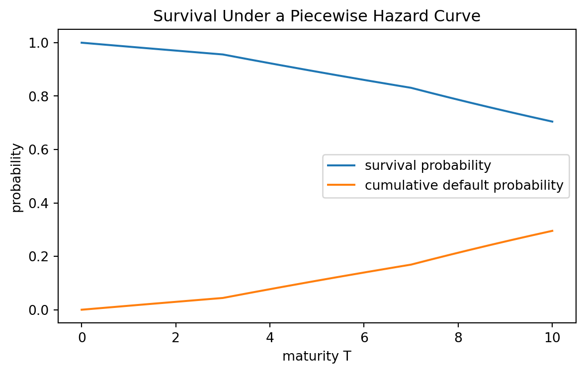
If $\lambda_t$ is deterministic, then
$$
\mathbb Q(\tau>T)=\exp\left(-\int_0^T\lambda_t\,dt\right).
$$
If $\lambda_t$ is stochastic, then the conditional survival probability has the form
$$
\mathbb Q(\tau>T\mid\mathcal F_t)
=
\mathbf 1_{\{\tau>t\}}
\mathbb E_t^{\mathbb Q}\left[
\exp\left(-\int_t^T\lambda_u\,du\right)
\right]
$$
under standard Cox-process assumptions.
::: {.definition}
## Intensity process
A default time $\tau$ has **intensity** $\lambda_t$ if the compensated default process
$$
M_t=H_t-\int_0^{t\wedge \tau}\lambda_s\,ds
$$
is a martingale.
:::
This is the credit-risk analogue of a compensated Poisson process. Before default, the process accumulates hazard. At default, the indicator jumps from $0$ to $1$.
::: {.theorem}
## Survival under deterministic intensity
If the hazard rate $\lambda(t)$ is deterministic and nonnegative, then
$$
S(T)=\mathbb Q(\tau>T)=\exp\left(-\int_0^T\lambda(t)\,dt\right).
$$
:::
::: {.proof-sketch}
The conditional default probability over a short interval is approximately $\lambda(t)dt$. Thus
$$
S(t+dt)\approx S(t)(1-\lambda(t)dt).
$$
Therefore
$$
\frac{S(t+dt)-S(t)}{dt}\approx -\lambda(t)S(t).
$$
Taking the limit gives the differential equation
$$
S'(t)=-\lambda(t)S(t),
\qquad S(0)=1.
$$
Solving this differential equation gives
$$
S(T)=\exp\left(-\int_0^T\lambda(t)\,dt\right).
$$
:::
```{python}
import numpy as np
import matplotlib.pyplot as plt

# Piecewise deterministic annual hazard curve.
T_grid = np.linspace(0, 10, 501)
lambda_grid = np.where(T_grid <= 3, 0.015, np.where(T_grid <= 7, 0.035, 0.055))

# Numerical cumulative hazard: integral of lambda(t) dt.
dt = T_grid[1] - T_grid[0]
cumulative_hazard = np.cumsum(lambda_grid) * dt
survival = np.exp(-cumulative_hazard)
default_probability = 1 - survival

plt.figure(figsize=(7, 4))
plt.plot(T_grid, survival, label="survival probability")
plt.plot(T_grid, default_probability, label="cumulative default probability")
plt.xlabel("maturity T")
plt.ylabel("probability")
plt.title("Survival Under a Piecewise Hazard Curve")
plt.legend()
plt.show()
```
## 29.9 Pricing with Default Intensity
Consider a defaultable payoff $X_T$ that is paid only if the borrower survives to $T$. If default gives zero recovery, the time-zero price is
$$
V_0
=
\mathbb E^{\mathbb Q}\left[e^{-\int_0^T r_u\,du}X_T\mathbf 1_{\{\tau>T\}}\right].
$$
If default is independent of market factors and $r$ and $\lambda$ are deterministic, this becomes
$$
V_0
=
e^{-\int_0^T (r_u+\lambda_u)\,du}\mathbb E^{\mathbb Q}[X_T].
$$
Thus default intensity acts like an additional discount rate.
With fractional recovery of market value, the risky discount rate becomes
$$
r_t+(1-R)\lambda_t.
$$
This leads to the pricing expression
$$
V_0
=
\mathbb E^{\mathbb Q}\left[
\exp\left(-\int_0^T (r_u+(1-R)\lambda_u)\,du\right)X_T
\right]
$$
in a simplified setting.
::: {.remark}
## Credit valuation adjustment intuition
For counterparty credit risk, the defaultable value is often written as risk-free value minus a credit valuation adjustment:
$$
V^{\mathrm{defaultable}}=V^{\mathrm{risk-free}}-CVA.
$$
A simple unilateral CVA formula has the approximate structure
$$
CVA\approx \mathbb E^{\mathbb Q}\left[\int_0^T e^{-\int_0^t r_u\,du}LGD\cdot EE_t\cdot \lambda_t S(t)\,dt\right],
$$
where $EE_t$ is expected positive exposure. This formula shows why credit risk combines exposure, default likelihood, and loss severity.
:::
## 29.10 Credit Default Swaps
A **credit default swap** is a contract in which a protection buyer pays periodic premiums to a protection seller. If default occurs, the seller pays a default compensation, often approximately equal to $LGD=1-R$ times notional.
The CDS par spread is chosen so that the present value of the premium leg equals the present value of the protection leg.
Suppose premiums are paid at dates
$$
0<t_1<t_2<\cdots<t_n=T,
$$
with year fractions $\Delta_i=t_i-t_{i-1}$. Let
$$
D_i=e^{-rt_i},
\qquad
S_i=\mathbb Q(\tau>t_i).
$$
A simple premium leg approximation is
$$
PV_{\mathrm{prem}}(c)
= c\sum_{i=1}^n \Delta_i D_i S_i.
$$
A simple protection leg approximation is
$$
PV_{\mathrm{prot}}
= (1-R)\sum_{i=1}^n D_i(S_{i-1}-S_i).
$$
The par spread $c^*$ satisfies
$$
PV_{\mathrm{prem}}(c^*)=PV_{\mathrm{prot}},
$$
so
$$
c^*=
\frac{(1-R)\sum_{i=1}^n D_i(S_{i-1}-S_i)}
{\sum_{i=1}^n \Delta_i D_i S_i}.
$$
For small time steps and constant $r,\lambda,R$, this is close to
$$
c^*\approx (1-R)\lambda.
$$
```{python}
import numpy as np

def cds_par_spread(T=5.0, r=0.04, lam=0.03, R=0.40, payments_per_year=4):
    n = int(T * payments_per_year)
    times = np.arange(1, n + 1) / payments_per_year
    delta = 1 / payments_per_year
    disc = np.exp(-r * times)
    surv = np.exp(-lam * times)
    surv_prev = np.r_[1.0, surv[:-1]]
    premium_annuity = np.sum(delta * disc * surv)
    protection_leg = (1 - R) * np.sum(disc * (surv_prev - surv))
    return protection_leg / premium_annuity

for lam in [0.01, 0.03, 0.07, 0.12]:
    spread = cds_par_spread(lam=lam)
    approx = (1 - 0.40) * lam
    print(f"lambda={lam:0.2%}, CDS spread={10000*spread:7.2f} bps, approx={10000*approx:7.2f} bps")
```
::: {.ai-box}
## AI-assisted checkpoint: CDS formula audit
Ask an AI tool to explain the CDS par spread formula above. Then check whether the explanation correctly distinguishes:
1. the premium leg from the protection leg;
2. survival probabilities $S_i$ from default probabilities $S_{i-1}-S_i$;
3. discount factors $D_i$ from survival factors $S_i$;
4. the exact discrete formula from the approximation $c\approx(1-R)\lambda$.
A good answer should explicitly say that the approximation depends on modeling assumptions and payment frequency.
:::
## 29.11 Rating Transition Matrices
Credit risk can also be modeled through rating migrations. Let the possible states be
$$
AAA, AA, A, BBB, BB, B, D,
$$
where $D$ is default. A transition matrix $P$ has entries
$$
P_{ij}=\mathbb P(X_{t+1}=j\mid X_t=i).
$$
The default state is usually absorbing:
$$
P_{DD}=1.
$$
If the current rating distribution is a row vector $\pi_0$, then after $n$ years,
$$
\pi_n=\pi_0P^n.
$$
The $n$-year default probability for a firm initially in rating $i$ is the entry of $P^n$ corresponding to state $D$.
```{python}
import numpy as np
import pandas as pd

ratings = ["AAA", "AA", "A", "BBB", "BB", "B", "D"]
P = np.array([
    [0.90, 0.08, 0.015, 0.003, 0.001, 0.0005, 0.0005],
    [0.02, 0.90, 0.060, 0.015, 0.003, 0.0010, 0.0010],
    [0.005,0.04, 0.900, 0.040, 0.010, 0.0030, 0.0020],
    [0.001,0.01, 0.060, 0.860, 0.050, 0.0120, 0.0070],
    [0.000,0.003,0.012, 0.070, 0.800, 0.0800, 0.0350],
    [0.000,0.001,0.004, 0.015, 0.100, 0.7600, 0.1200],
    [0.000,0.000,0.000, 0.000, 0.000, 0.0000, 1.0000],
])

# Normalize rows in case of rounding.
P = P / P.sum(axis=1, keepdims=True)

rows = []
for start_rating in ["A", "BBB", "BB", "B"]:
    i = ratings.index(start_rating)
    for n in [1, 2, 3, 5, 10]:
        Pn = np.linalg.matrix_power(P, n)
        default_prob = Pn[i, ratings.index("D")]
        rows.append({"initial_rating": start_rating, "years": n, "default_probability": default_prob})

pd.DataFrame(rows).round(4)
```
## 29.12 Portfolio Credit Risk
For a portfolio with $m$ obligors, a simple default-loss model is
$$
L=\sum_{i=1}^m EAD_i\cdot LGD_i\cdot \mathbf 1_{\{\tau_i\le T\}}.
$$
Even if single-name default probabilities are known, the portfolio loss distribution depends strongly on default dependence.
### Independent Bernoulli defaults
If each obligor defaults independently with probability $p_i$, then
$$
\mathbf 1_{\{\tau_i\le T\}}\sim \operatorname{Bernoulli}(p_i).
$$
The expected loss is
$$
\mathbb E[L]=\sum_{i=1}^m EAD_i\cdot LGD_i\cdot p_i.
$$
The variance under independence is
$$
\operatorname{Var}(L)
=\sum_{i=1}^m (EAD_iLGD_i)^2 p_i(1-p_i).
$$
### Correlated defaults
Defaults are not independent in stress periods. A common one-factor Gaussian threshold model is:
$$
Y_i=\sqrt{\rho}\,Z+\sqrt{1-\rho}\,\varepsilon_i,
$$
where $Z$ is a common factor and $\varepsilon_i$ are idiosyncratic shocks. Obligor $i$ defaults if
$$
Y_i\le \Phi^{-1}(p_i).
$$
The parameter $\rho$ controls default correlation. Higher $\rho$ usually increases tail risk even when expected loss stays roughly the same.
```{python}
import numpy as np

rng = np.random.default_rng(7243)

m = 200
n_sim = 50_000
EAD = np.full(m, 1.0)
LGD = np.full(m, 0.60)
p = np.full(m, 0.02)

# For p = 2%, the threshold is approximately -2.0537.
# We use a constant to avoid relying on scipy in the book example.
threshold = -2.053748910631823

def simulate_losses(rho):
    Z = rng.normal(size=(n_sim, 1))
    eps = rng.normal(size=(n_sim, m))
    Y = np.sqrt(rho) * Z + np.sqrt(1 - rho) * eps
    defaults = Y <= threshold
    losses = defaults @ (EAD * LGD)
    return losses

for rho in [0.0, 0.1, 0.3, 0.6]:
    losses = simulate_losses(rho)
    var_99 = np.quantile(losses, 0.99)
    es_99 = losses[losses >= var_99].mean()
    print(f"rho={rho:0.1f}: mean={losses.mean():0.2f}, VaR99={var_99:0.2f}, ES99={es_99:0.2f}")
```
::: {.remark}
## Correlation is a tail-risk parameter
In credit portfolios, default correlation may have a modest effect on expected loss but a large effect on tail loss. This is why credit portfolio models must be assessed with VaR, Expected Shortfall, stress testing, and scenario analysis, not only average losses.
:::
## 29.13 Credit Risk and Martingale Pricing
Credit-risk pricing fits the general framework of this book. Under a risk-neutral measure $\mathbb Q$, a defaultable payoff has price
$$
V_t
=
\mathbb E_t^{\mathbb Q}\left[
\exp\left(-\int_t^T r_u\,du\right)X_T\right],
$$
where $X_T$ includes survival and recovery terms.
For example, if a claim pays $1$ at $T$ only if no default has occurred, then
$$
X_T=\mathbf 1_{\{\tau>T\}}.
$$
The price is
$$
V_0=\mathbb E^{\mathbb Q}\left[e^{-\int_0^T r_u\,du}\mathbf 1_{\{\tau>T\}}\right].
$$
If $r$ and $\lambda$ are deterministic, then
$$
V_0=\exp\left(-\int_0^T (r_u+\lambda_u)\,du\right).
$$
Thus the default intensity appears as an additional discounting term. This is the same martingale-pricing principle that appeared in option pricing, but with a jump-to-default event.
## 29.14 Model Risk in Credit Models
Credit-risk models are sensitive to assumptions:
- Default probabilities may be estimated from limited historical data.
- Recoveries are random and often correlated with default rates.
- Defaults are strongly dependent in crises.
- Market spreads include risk premia and liquidity effects.
- Structural models require unobservable firm asset values and volatilities.
- Reduced-form models may fit spreads without explaining economic default mechanisms.
::: {.ai-box}
## AI-assisted model critique
Ask an AI tool to compare the Merton model and a reduced-form intensity model for corporate bond pricing. Then check whether the answer mentions all of the following:
- Merton default is driven by firm asset value and debt;
- reduced-form default is modeled directly through an intensity;
- Merton equity is naturally interpreted as a call option;
- intensity models are often easier to calibrate to CDS or bond spreads;
- both models require assumptions under $\mathbb Q$ for pricing;
- neither model alone captures all real credit-market effects.
:::
## 29.15 Common Mistakes
1. **Using physical default probabilities for pricing without adjustment.** Pricing defaultable securities requires risk-neutral inputs or a pricing kernel.
2. **Forgetting recovery.** Default does not always mean zero payoff.
3. **Treating $s=(1-R)\lambda$ as universal.** This relationship depends on conventions and approximations.
4. **Ignoring default dependence.** Portfolio credit risk is dominated by dependence in the tail.
5. **Confusing spread with expected loss.** Spreads include risk premia and market frictions.
6. **Using a rating transition matrix without checking the horizon.** One-year transition matrices must be compounded or otherwise transformed for longer horizons.
7. **Mixing pre-default and post-default values.** Defaultable claims often have jumps at default.
## 29.16 Python Summary: A Small Credit Dashboard
The following example combines hazard rates, recovery, risky bond spreads, and expected loss.
```{python}
import numpy as np
import pandas as pd

names = ["Firm A", "Firm B", "Firm C", "Firm D"]
EAD = np.array([10.0, 15.0, 8.0, 12.0])       # millions
LGD = np.array([0.45, 0.60, 0.35, 0.70])
lambda_Q = np.array([0.012, 0.030, 0.018, 0.055])
lambda_P = np.array([0.007, 0.018, 0.010, 0.035])
T = 1.0
r = 0.04

pd_physical = 1 - np.exp(-lambda_P * T)
pd_risk_neutral = 1 - np.exp(-lambda_Q * T)
expected_loss = EAD * LGD * pd_physical
approx_spread_bps = 10000 * LGD * lambda_Q
risky_zcb_price = np.exp(-r * T) * (1 - LGD * pd_risk_neutral)

credit_dashboard = pd.DataFrame({
    "name": names,
    "EAD_millions": EAD,
    "LGD": LGD,
    "PD_physical": pd_physical,
    "PD_risk_neutral": pd_risk_neutral,
    "expected_loss_millions": expected_loss,
    "approx_spread_bps": approx_spread_bps,
    "one_year_risky_ZCB_price": risky_zcb_price,
})

credit_dashboard.round(4)
```
## 29.17 AI-Assisted Code Review Prompt
Use the following prompt to check a credit-risk implementation:
> I am implementing a credit-risk model with default probability, recovery, hazard rates, risky bond prices, CDS spreads, and portfolio credit losses. Please audit the code for sign mistakes, missing discount factors, confusion between physical and risk-neutral probabilities, incorrect recovery conventions, and misuse of independence assumptions. Do not rewrite the code first. First list the assumptions required by each formula, then identify possible errors.
A useful AI answer should not merely say that the code is correct. It should identify the probability measure, recovery convention, time horizon, compounding convention, and dependence assumption used in each calculation.
## 29.18 Exercises
### Conceptual Exercises
1. Explain the difference between default probability, hazard rate, and credit spread.
2. Explain why the one-year default probability is $1-e^{-\lambda}$ under a constant hazard rate $\lambda$.
3. Why are risk-neutral default probabilities usually different from historical default frequencies?
4. What does recovery rate mean? Give two different recovery conventions.
5. Explain why credit spread is not the same as expected loss.
### Mathematical Exercises
6. Let $\lambda(t)=a+bt$ with $a,b\ge 0$. Derive $S(T)$.
7. Under recovery-at-maturity with constant $r$, $R$, and $\lambda$, derive
$$
P^{\mathrm{risk}}(0,T)=e^{-rT}\left(R+(1-R)e^{-\lambda T}\right).
$$
8. Show that for small $T$ and small $\lambda T$, the risky zero-coupon spread approximately satisfies
$$
s(T)\approx (1-R)\lambda.
$$
9. In the Merton model, derive the risk-neutral default probability $N(-d_2)$.
10. Show that risky debt in the Merton model can be written as risk-free debt minus a put option on firm value.
### Computational Exercises
11. Write Python code to plot $S(T)$ and $F(T)$ for constant hazard rates $1\%$, $3\%$, $7\%$, and $12\%$.
12. Compute risky zero-coupon bond prices for maturities $1,2,5,10$ using recovery rates $20\%,40\%,60\%$.
13. Implement the CDS par spread formula for quarterly payments and compare it with $(1-R)\lambda$.
14. Use a rating transition matrix to compute three-year and five-year default probabilities.
15. Simulate a portfolio of $100$ loans under independent Bernoulli defaults and estimate VaR and ES.
16. Repeat the previous exercise using a one-factor Gaussian model with $\rho=0.3$. Compare the tail risk.
### AI-Assisted Exercises
17. Ask an AI tool to explain why default correlation affects credit VaR more than expected loss. Check the explanation using a small simulation.
18. Ask an AI tool to derive the Merton model default probability. Identify where the normal distribution enters.
19. Give an AI tool a CDS pricing formula with a deliberate missing discount factor. Ask it to audit the formula.
20. Ask an AI tool to distinguish historical PD, risk-neutral PD, and rating-agency default frequency. Rewrite the answer in your own words.
## 29.19 Chapter Summary
Credit risk introduces a new financial event: default. The main mathematical object is the default time $\tau$. From $\tau$ we obtain survival probabilities, default probabilities, intensities, and loss distributions.
The chapter developed two major modeling viewpoints:
- **Structural models**, where default is caused by firm value falling below debt obligations;
- **Reduced-form models**, where default is modeled directly through an intensity process.
For pricing, credit-risk cash flows are discounted under the risk-neutral measure and must include survival and recovery terms. For risk management, portfolio credit losses depend not only on marginal default probabilities but also on default dependence. This is why credit risk connects probability, stochastic processes, option pricing, fixed income, and tail-risk measurement.