---
title: "Chapter 7. Random Variables, Distributions, and Financial Returns"
---
::: {.chapter-objectives}
## Learning Goals
By the end of this chapter, students should be able to:
- model one-period and multi-period returns as random variables;
- distinguish prices, simple returns, gross returns, and log returns;
- compute expectation, variance, covariance, skewness, and kurtosis of return distributions;
- explain why log returns are mathematically convenient for multi-period models;
- derive the connection between normal log returns and lognormal prices;
- identify the limitations of the normal model for financial returns;
- explain heavy tails, tail probabilities, quantiles, and downside risk;
- use empirical distributions, histograms, QQ plots, and Monte Carlo simulation to study returns;
- write Python code for return transformations and distribution diagnostics;
- use AI tools carefully to critique assumptions, check formulas, and audit numerical finance code.
:::
::: {.hero-box}
In finance, randomness enters through **future prices** and **future cash flows**. A return is therefore not just a number; before it is observed, it is a **random variable**.
The central object of this chapter is the log return
$$
X_t=\log\frac{S_t}{S_{t-1}}.
$$
Log returns add across time, while simple returns compound multiplicatively. This small algebraic difference is one reason that probability theory, statistics, and stochastic processes enter mathematical finance so naturally.
:::
## 7.1 From Deterministic Prices to Random Returns
In Chapters 1--6, we studied prices, payoffs, arbitrage, risk-neutral probabilities, and martingales in finite models. We now pause to build the probability language needed for the next part of the book.
Let $S_t$ denote the price of an asset at time $t$. At the beginning of a time period, $S_t$ may be known, but $S_{t+1}$ is usually uncertain. Therefore $S_{t+1}$ is modeled as a random variable.
The simple return from $t$ to $t+1$ is
$$
R_{t+1}=\frac{S_{t+1}-S_t}{S_t}.
$$
Equivalently,
$$
S_{t+1}=S_t(1+R_{t+1}).
$$
The gross return is
$$
G_{t+1}=1+R_{t+1}=\frac{S_{t+1}}{S_t}.
$$
The log return is
$$
X_{t+1}=\log G_{t+1}=\log\frac{S_{t+1}}{S_t}.
$$
Thus
$$
G_{t+1}=e^{X_{t+1}},
\qquad
R_{t+1}=e^{X_{t+1}}-1.
$$
For small returns, $X_{t+1}$ and $R_{t+1}$ are close because
$$
\log(1+r)=r-\frac{r^2}{2}+\frac{r^3}{3}-\cdots.
$$
But they are not the same object. The difference becomes important for volatility, tail risk, multi-period aggregation, and model calibration.
::: {.warning}
A common mistake is to average simple returns and log returns interchangeably. Simple returns are natural for portfolio values over one period. Log returns are natural for time aggregation. They answer different mathematical questions.
:::
## 7.2 Random Variables and Distributions
A random variable is a measurable function
$$
X:\Omega\to\mathbb R.
$$
In financial applications, $X$ may represent a return, a loss, a payoff, a risk factor, an interest-rate change, or a trading profit.
The distribution of $X$ is the probability law of its possible values. It can be described by the cumulative distribution function
$$
F_X(x)=\mathbb P(X\le x).
$$
If $X$ is discrete with values $x_1,\ldots,x_m$, then its probability mass function is
$$
p_i=\mathbb P(X=x_i),
\qquad i=1,\ldots,m.
$$
If $X$ has a density $f_X$, then
$$
F_X(x)=\int_{-\infty}^x f_X(u)\,du.
$$
In finance, the distribution matters because pricing, risk measurement, and portfolio construction all depend on how likely different future outcomes are.
For example:
- the mean return summarizes central tendency;
- the variance measures dispersion;
- the lower tail determines downside risk;
- high quantiles of loss distributions determine risk capital;
- dependence between returns determines diversification.
## 7.3 Simple Returns, Gross Returns, and Log Returns
Assume $S_t>0$ for all $t$. Define
$$
R_t=\frac{S_t-S_{t-1}}{S_{t-1}},
\qquad
G_t=1+R_t=\frac{S_t}{S_{t-1}},
\qquad
X_t=\log G_t.
$$
The multi-period gross return from time $0$ to time $n$ is
$$
\frac{S_n}{S_0}
=
\frac{S_1}{S_0}\frac{S_2}{S_1}\cdots\frac{S_n}{S_{n-1}}
=
\prod_{t=1}^n G_t.
$$
Taking logarithms gives
$$
\log\frac{S_n}{S_0}
=
\sum_{t=1}^n \log G_t
=
\sum_{t=1}^n X_t.
$$
This is the main algebraic reason that log returns are useful.
::: {.theorem}
### Theorem 7.1: Additivity of log returns
If $S_t>0$ for $t=0,1,\ldots,n$, then
$$
\log\frac{S_n}{S_0}=\sum_{t=1}^n \log\frac{S_t}{S_{t-1}}.
$$
:::
::: {.proof}
By telescoping,
$$
\frac{S_n}{S_0}
=
\prod_{t=1}^n \frac{S_t}{S_{t-1}}.
$$
Taking logarithms and using $\log(ab)=\log a+\log b$ gives the result.
:::
The corresponding relation for simple returns is multiplicative:
$$
1+R_{0,n}
=
\prod_{t=1}^n (1+R_t),
$$
where
$$
R_{0,n}=\frac{S_n-S_0}{S_0}.
$$
Therefore the multi-period simple return is
$$
R_{0,n}=\prod_{t=1}^n (1+R_t)-1.
$$
This difference between addition and multiplication is fundamental.
## 7.4 Interactive Demo: Simple Returns versus Log Returns
The following Plotly.js activity compares the simple return $R$, gross return $1+R$, and log return $X=\log(1+R)$.
::: {.interactive-card}
### Interactive 7.1: Return transformations
Move the slider to see how simple returns and log returns differ. The approximation $\log(1+r)\approx r$ is accurate near zero, but not in the tails.
<div class="mf-controls">
<label for="mf-ch07-return-slider">Simple return $r$</label>
<input id="mf-ch07-return-slider" type="range" min="-0.9" max="1.0" step="0.01" value="0.10">
<span id="mf-ch07-return-value">0.10</span>
</div>
<div id="mf-ch07-return-plot" class="plotly-demo"></div>
<div id="mf-ch07-return-output" class="mf-output"></div>
<script>
document.addEventListener("DOMContentLoaded", function() {
const slider = document.getElementById("mf-ch07-return-slider");
const value = document.getElementById("mf-ch07-return-value");
const output = document.getElementById("mf-ch07-return-output");
const plot = document.getElementById("mf-ch07-return-plot");
if (!slider || !plot || typeof Plotly === "undefined") return;
const grid = [];
for (let i = -90; i <= 100; i++) grid.push(i / 100);
const logVals = grid.map(r => Math.log(1 + r));
const approxVals = grid.map(r => r);
function draw() {
const r = Number(slider.value);
const x = Math.log(1 + r);
value.textContent = r.toFixed(2);
output.innerHTML = `Gross return: <b>${(1+r).toFixed(4)}</b> | Log return: <b>${x.toFixed(4)}</b> | Difference r - log(1+r): <b>${(r-x).toFixed(4)}</b>`;
const traces = [
{
x: grid,
y: logVals,
mode: "lines",
name: "x = log(1+r)",
line: {width: 3}
},
{
x: grid,
y: approxVals,
mode: "lines",
name: "x = r",
line: {dash: "dash", width: 2}
},
{
x: [r],
y: [x],
mode: "markers",
name: "selected return",
marker: {size: 12}
}
];
const layout = {
margin: {l: 55, r: 25, t: 35, b: 55},
xaxis: {title: "simple return r", zeroline: true},
yaxis: {title: "log return", zeroline: true},
legend: {orientation: "h"}
};
Plotly.react(plot, traces, layout, {responsive: true});
}
slider.addEventListener("input", draw);
draw();
});
</script>
:::
## 7.5 Moments of Return Distributions
Let $X$ be a return random variable. Its expectation is
$$
\mathbb E[X]=\int x\,dF_X(x),
$$
or, in a finite model,
$$
\mathbb E[X]=\sum_{i=1}^m x_i p_i.
$$
The variance is
$$
\operatorname{Var}(X)=\mathbb E[(X-\mathbb E[X])^2].
$$
Equivalently,
$$
\operatorname{Var}(X)=\mathbb E[X^2]-(\mathbb E[X])^2.
$$
The standard deviation is
$$
\sigma_X=\sqrt{\operatorname{Var}(X)}.
$$
In finance, the standard deviation of returns is called **volatility**. Volatility measures the scale of fluctuations, but it does not by itself distinguish upside volatility from downside volatility.
The third central moment measures asymmetry:
$$
\mu_3=\mathbb E[(X-\mu)^3],
\qquad \mu=\mathbb E[X].
$$
The skewness is
$$
\gamma_1=\frac{\mathbb E[(X-\mu)^3]}{\sigma^3}.
$$
The fourth central moment measures tail thickness:
$$
\mu_4=\mathbb E[(X-\mu)^4].
$$
The kurtosis is
$$
\gamma_2=\frac{\mathbb E[(X-\mu)^4]}{\sigma^4}.
$$
The normal distribution has kurtosis $3$. Therefore the excess kurtosis is
$$
\gamma_2-3.
$$
Financial returns often exhibit negative skewness and positive excess kurtosis. This means large losses may occur more often than a normal model predicts.
::: {.definition}
### Definition 7.1: Volatility
If $R$ is a return over a fixed time period, its volatility is the standard deviation
$$
\sigma_R=\sqrt{\operatorname{Var}(R)}.
$$
If returns are measured daily and are independent with common variance, annualized volatility is often approximated by
$$
\sigma_{\mathrm{ann}}=\sqrt{252}\,\sigma_{\mathrm{daily}}.
$$
:::
The square-root-of-time rule should be used carefully. It depends on assumptions such as independence and constant variance.
## 7.6 Worked Example: A Three-State Return Distribution
Suppose a one-period simple return $R$ has the following distribution:
| State | Return $r_i$ | Probability $p_i$ |
|---:|---:|---:|
| Down | $-0.20$ | $0.25$ |
| Middle | $0.05$ | $0.50$ |
| Up | $0.30$ | $0.25$ |
The expected return is
$$
\mathbb E[R]
=
(-0.20)(0.25)+(0.05)(0.50)+(0.30)(0.25)
=0.05.
$$
The second moment is
$$
\mathbb E[R^2]
=(0.04)(0.25)+(0.0025)(0.50)+(0.09)(0.25)
=0.03375.
$$
Therefore
$$
\operatorname{Var}(R)=0.03375-(0.05)^2=0.03125,
$$
and
$$
\sigma_R=\sqrt{0.03125}\approx 0.1768.
$$
This example shows why the expected return alone is not enough. Two assets may have the same expected return but very different dispersion and tail risk.
```{python}
#| label: ch07-three-state-moments
#| fig-cap: "Moment calculations for a three-state return distribution."
import numpy as np
import pandas as pd

states = np.array(["Down", "Middle", "Up"])
returns = np.array([-0.20, 0.05, 0.30])
prob = np.array([0.25, 0.50, 0.25])

mu = np.sum(prob * returns)
second_moment = np.sum(prob * returns**2)
var = second_moment - mu**2
sd = np.sqrt(var)
skew = np.sum(prob * (returns - mu)**3) / sd**3
kurt = np.sum(prob * (returns - mu)**4) / sd**4

summary = pd.DataFrame({
    "quantity": ["mean", "second moment", "variance", "standard deviation", "skewness", "kurtosis"],
    "value": [mu, second_moment, var, sd, skew, kurt]
})
summary
```
## 7.7 Covariance, Correlation, and Diversification
For two return random variables $R_1$ and $R_2$, covariance is
$$
\operatorname{Cov}(R_1,R_2)
=\mathbb E[(R_1-\mu_1)(R_2-\mu_2)],
$$
where
$$
\mu_i=\mathbb E[R_i].
$$
Correlation is the normalized covariance:
$$
\rho_{12}=\frac{\operatorname{Cov}(R_1,R_2)}{\sigma_1\sigma_2}.
$$
If a portfolio has weights $w_1$ and $w_2$, its return is
$$
R_p=w_1R_1+w_2R_2.
$$
Its expected return is
$$
\mathbb E[R_p]=w_1\mathbb E[R_1]+w_2\mathbb E[R_2],
$$
and its variance is
$$
\operatorname{Var}(R_p)
=
w_1^2\sigma_1^2+w_2^2\sigma_2^2+2w_1w_2\sigma_1\sigma_2\rho_{12}.
$$
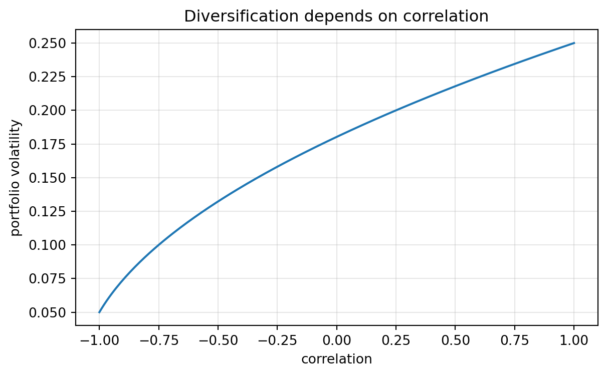
The covariance term is the mathematical source of diversification. If $\rho_{12}<1$, the portfolio variance may be smaller than the weighted average of individual variances.
For $d$ assets with return vector
$$
R=(R_1,\ldots,R_d)^\top,
$$
mean vector
$$
\mu=\mathbb E[R],
$$
and covariance matrix
$$
\Sigma=\mathbb E[(R-\mu)(R-\mu)^\top],
$$
a portfolio with weight vector $w$ has return
$$
R_p=w^\top R,
$$
mean
$$
\mathbb E[R_p]=w^\top\mu,
$$
and variance
$$
\operatorname{Var}(R_p)=w^\top\Sigma w.
$$
This formula will become central in Chapter 26 on mean-variance portfolio theory.
```{python}
#| label: ch07-portfolio-variance
#| fig-cap: "Portfolio volatility as a function of correlation."
import numpy as np
import matplotlib.pyplot as plt

w1, w2 = 0.5, 0.5
sigma1, sigma2 = 0.20, 0.30
rho_grid = np.linspace(-1, 1, 201)
portfolio_var = (
    w1**2 * sigma1**2
    + w2**2 * sigma2**2
    + 2 * w1 * w2 * sigma1 * sigma2 * rho_grid
)
portfolio_sd = np.sqrt(portfolio_var)

plt.figure(figsize=(7, 4))
plt.plot(rho_grid, portfolio_sd)
plt.xlabel("correlation")
plt.ylabel("portfolio volatility")
plt.title("Diversification depends on correlation")
plt.grid(True, alpha=0.3)
plt.show()
```
## 7.8 Normal Returns and the Normal Model
A common first model assumes that a return variable is normally distributed:
$$
X\sim N(\mu,\sigma^2).
$$
This means that $X$ has density
$$
f_X(x)=\frac{1}{\sigma\sqrt{2\pi}}
\exp\left(-\frac{(x-\mu)^2}{2\sigma^2}\right).
$$
The normal model is mathematically convenient because sums of independent normal variables are normal. If
$$
X_1,\ldots,X_n
$$
are independent and
$$
X_t\sim N(\mu_t,\sigma_t^2),
$$
then
$$
\sum_{t=1}^n X_t\sim
N\left(\sum_{t=1}^n\mu_t,\sum_{t=1}^n\sigma_t^2\right).
$$
In particular, if $X_t$ are independent and identically distributed as $N(\mu,\sigma^2)$, then
$$
\sum_{t=1}^n X_t\sim N(n\mu,n\sigma^2).
$$
This matches the additivity of log returns.
::: {.theorem}
### Theorem 7.2: Aggregation of independent normal log returns
Suppose $X_1,\ldots,X_n$ are independent log returns with
$$
X_t\sim N(\mu,\sigma^2).
$$
Then the cumulative log return is
$$
X_{1:n}=\sum_{t=1}^n X_t\sim N(n\mu,n\sigma^2).
$$
Therefore
$$
\log\frac{S_n}{S_0}\sim N(n\mu,n\sigma^2).
$$
:::
This theorem is one of the basic probabilistic justifications for geometric Brownian motion in continuous time.
## 7.9 Lognormal Prices
If log returns are normal, then prices are lognormal. Suppose
$$
\log\frac{S_T}{S_0}=X\sim N(m,v).
$$
Then
$$
S_T=S_0e^X.
$$
A positive random variable $Y$ is lognormal if $\log Y$ is normal. Thus $S_T$ is lognormal.
The expectation of $e^X$ for $X\sim N(m,v)$ is
$$
\mathbb E[e^X]=e^{m+v/2}.
$$
Therefore
$$
\mathbb E[S_T]=S_0e^{m+v/2}.
$$
This correction term $v/2$ is important. It appears again in geometric Brownian motion, Itô's formula, and the Black--Scholes model.
::: {.theorem}
### Theorem 7.3: Normal log returns imply lognormal prices
If
$$
X=\log\frac{S_T}{S_0}\sim N(m,v),
$$
then
$$
S_T=S_0e^X
$$
is lognormally distributed and
$$
\mathbb E[S_T]=S_0e^{m+v/2}.
$$
:::
::: {.proof}
Since $S_T=S_0e^X$, we have
$$
\log S_T=\log S_0+X.
$$
A constant plus a normal random variable is normal. Hence $\log S_T$ is normal, so $S_T$ is lognormal.
The expectation follows from the moment generating function of a normal random variable:
$$
\mathbb E[e^{uX}]=\exp\left(um+\frac12u^2v\right).
$$
Set $u=1$ and multiply by $S_0$.
:::
::: {.warning}
If $X$ is normal, then $R=e^X-1$ is not normal. Normal log returns imply lognormal gross returns and simple returns bounded below by $-1$.
:::
## 7.10 Interactive Demo: Normal Log Returns and Lognormal Prices
::: {.interactive-card}
### Interactive 7.2: Simulated terminal prices under normal log returns
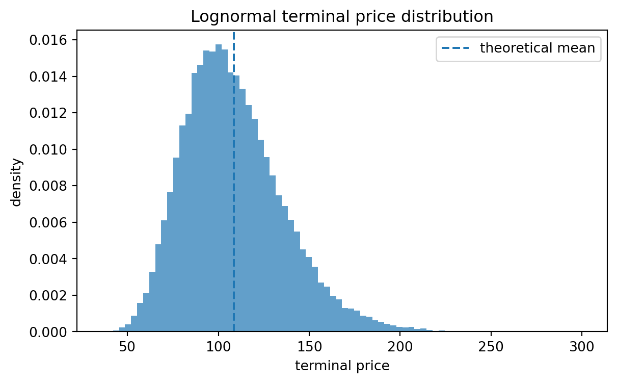
Adjust the mean and volatility of log returns. The left panel shows the log-return distribution. The right panel shows the resulting terminal price distribution. Notice that the price distribution is positive and skewed.
<div class="mf-controls">
<label for="mf-ch07-mu-slider">Mean log return $m$</label>
<input id="mf-ch07-mu-slider" type="range" min="-0.20" max="0.20" step="0.01" value="0.05">
<span id="mf-ch07-mu-value">0.05</span>
<label for="mf-ch07-vol-slider">Volatility $\sqrt v$</label>
<input id="mf-ch07-vol-slider" type="range" min="0.05" max="0.80" step="0.01" value="0.25">
<span id="mf-ch07-vol-value">0.25</span>
</div>
<div id="mf-ch07-lognormal-plot" class="plotly-demo"></div>
<div id="mf-ch07-lognormal-output" class="mf-output"></div>
<script>
document.addEventListener("DOMContentLoaded", function() {
const muSlider = document.getElementById("mf-ch07-mu-slider");
const volSlider = document.getElementById("mf-ch07-vol-slider");
const muValue = document.getElementById("mf-ch07-mu-value");
const volValue = document.getElementById("mf-ch07-vol-value");
const output = document.getElementById("mf-ch07-lognormal-output");
const plot = document.getElementById("mf-ch07-lognormal-plot");
if (!muSlider || !volSlider || !plot || typeof Plotly === "undefined") return;
const s0 = 100;
function normalPdf(x, mu, sigma) {
return Math.exp(-0.5 * Math.pow((x - mu) / sigma, 2)) / (sigma * Math.sqrt(2 * Math.PI));
}
function lognormalPdf(s, s0, mu, sigma) {
if (s <= 0) return 0;
const z = Math.log(s / s0);
return normalPdf(z, mu, sigma) / s;
}
function linspace(a, b, n) {
const arr = [];
for (let i = 0; i < n; i++) arr.push(a + (b - a) * i / (n - 1));
return arr;
}
function draw() {
const mu = Number(muSlider.value);
const sigma = Number(volSlider.value);
muValue.textContent = mu.toFixed(2);
volValue.textContent = sigma.toFixed(2);
const xGrid = linspace(mu - 4 * sigma, mu + 4 * sigma, 300);
const xPdf = xGrid.map(x => normalPdf(x, mu, sigma));
const sMax = Math.max(200, s0 * Math.exp(mu + 4 * sigma));
const sGrid = linspace(1, sMax, 300);
const sPdf = sGrid.map(s => lognormalPdf(s, s0, mu, sigma));
const expectedPrice = s0 * Math.exp(mu + 0.5 * sigma * sigma);
const medianPrice = s0 * Math.exp(mu);
const traces = [
{
x: xGrid,
y: xPdf,
mode: "lines",
name: "log return density",
xaxis: "x1",
yaxis: "y1",
line: {width: 3}
},
{
x: sGrid,
y: sPdf,
mode: "lines",
name: "terminal price density",
xaxis: "x2",
yaxis: "y2",
line: {width: 3}
},
{
x: [expectedPrice, expectedPrice],
y: [0, Math.max(...sPdf)],
mode: "lines",
name: "E[S_T]",
xaxis: "x2",
yaxis: "y2",
line: {dash: "dash", width: 2}
}
];
const layout = {
margin: {l: 50, r: 25, t: 35, b: 55},
grid: {rows: 1, columns: 2, pattern: "independent"},
xaxis: {title: "log return"},
yaxis: {title: "density"},
xaxis2: {title: "terminal price"},
yaxis2: {title: "density"},
legend: {orientation: "h"}
};
output.innerHTML = `With S0 = 100, median price = <b>${medianPrice.toFixed(2)}</b>, expected price = <b>${expectedPrice.toFixed(2)}</b>. The gap is caused by the variance correction.`;
Plotly.react(plot, traces, layout, {responsive: true});
}
muSlider.addEventListener("input", draw);
volSlider.addEventListener("input", draw);
draw();
});
</script>
:::
```{python}
#| label: ch07-lognormal-simulation
#| fig-cap: "Simulating lognormal terminal prices from normal log returns."
import numpy as np
import matplotlib.pyplot as plt

rng = np.random.default_rng(7243)
S0 = 100.0
m = 0.05
sigma = 0.25
n_sims = 50_000

X = rng.normal(loc=m, scale=sigma, size=n_sims)
ST = S0 * np.exp(X)

theoretical_mean = S0 * np.exp(m + 0.5 * sigma**2)
empirical_mean = ST.mean()
empirical_median = np.median(ST)

print("Theoretical E[S_T]:", round(theoretical_mean, 4))
print("Empirical mean:", round(empirical_mean, 4))
print("Empirical median:", round(empirical_median, 4))

plt.figure(figsize=(7, 4))
plt.hist(ST, bins=80, density=True, alpha=0.7)
plt.axvline(theoretical_mean, linestyle="--", label="theoretical mean")
plt.xlabel("terminal price")
plt.ylabel("density")
plt.title("Lognormal terminal price distribution")
plt.legend()
plt.show()
```
## 7.11 Tail Probabilities and Quantiles
Risk management often focuses on tails rather than averages. If $L$ is a loss random variable, a high value of $L$ is bad. The distribution function is
$$
F_L(x)=\mathbb P(L\le x).
$$
The $\alpha$-quantile is
$$
q_\alpha(L)=\inf\{x:F_L(x)\ge \alpha\}.
$$
For example, the $0.95$-quantile of the loss distribution is the level below which losses fall with probability at least $95\%$.
If $R$ is a return, then loss is often defined as
$$
L=-R.
$$
Large losses correspond to very negative returns.
A lower-tail return quantile is
$$
q_\alpha(R)=\inf\{x:F_R(x)\ge\alpha\},
$$
where $\alpha$ may be $0.01$ or $0.05$.
The lower $5\%$ return quantile answers the question:
> What return level is exceeded in approximately $95\%$ of periods, but breached in approximately $5\%$ of periods?
This idea will later lead to Value at Risk and Expected Shortfall in Chapter 28.
## 7.12 Heavy Tails
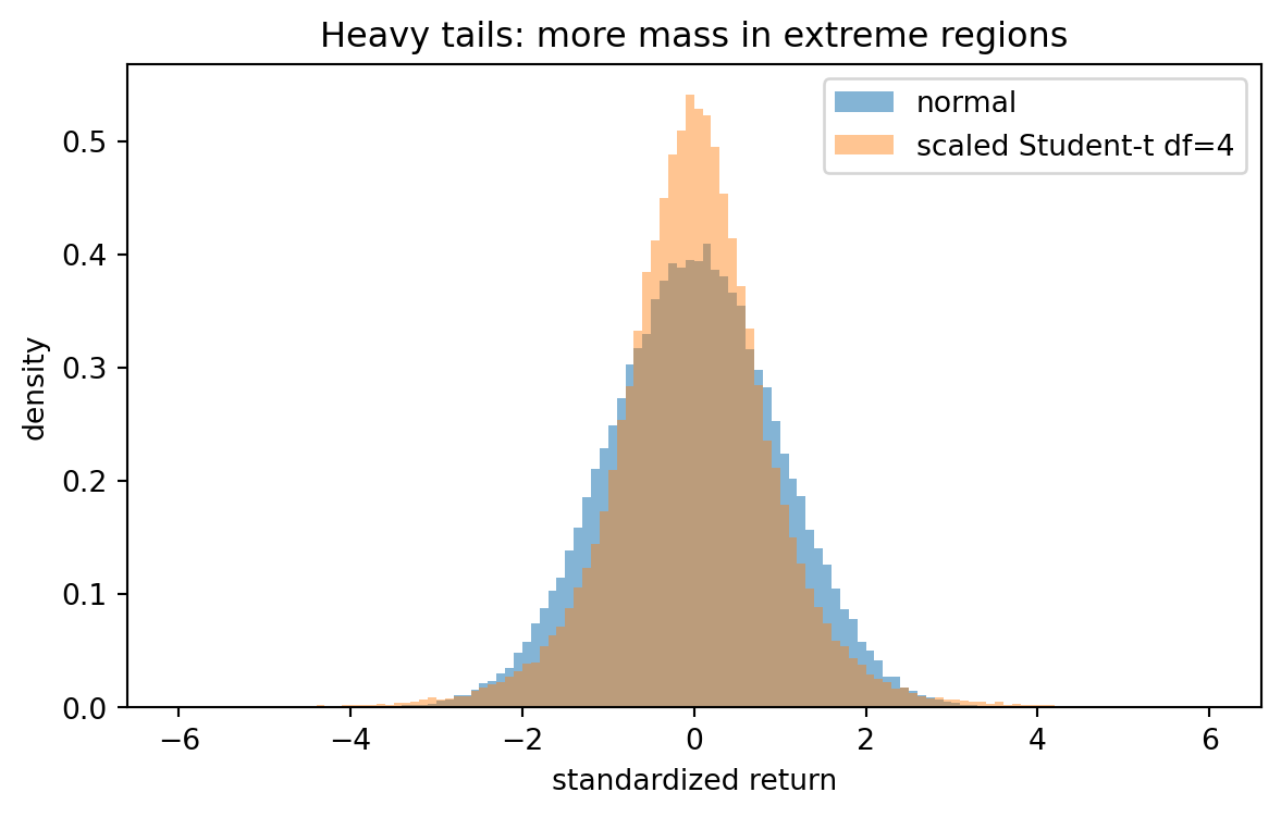
A distribution is said informally to have heavy tails if extreme observations occur more often than they would under a normal distribution with comparable mean and variance.
There are several mathematical ways to describe tail heaviness. One useful comparison is tail probability:
$$
\mathbb P(|X-\mu|>k\sigma).
$$
For a standard normal variable $Z\sim N(0,1)$,
$$
\mathbb P(|Z|>3)\approx 0.0027.
$$
In many financial return data sets, observations more than three sample standard deviations from the mean occur more often than this normal benchmark suggests.
Another way is through kurtosis. A distribution with excess kurtosis greater than zero has heavier tails than the normal distribution in the fourth-moment sense.
::: {.warning}
High kurtosis is not the same as tail risk in every possible sense. Kurtosis depends on the fourth moment. Some heavy-tailed distributions do not even have finite fourth moments.
:::
### Student-t returns
A common heavy-tailed model is the Student-t distribution. If $T_\nu$ has $\nu$ degrees of freedom, then it has heavier tails than the standard normal distribution. As $\nu\to\infty$, the Student-t distribution approaches the normal distribution.
The Student-t model is useful pedagogically because it shows that two distributions can have similar centers and scales but very different tail probabilities.
```{python}
#| label: ch07-heavy-tails
#| fig-cap: "Normal and Student-t samples can have very different tail behavior."
import numpy as np
import matplotlib.pyplot as plt

rng = np.random.default_rng(7339)
n = 100_000
normal_sample = rng.normal(size=n)
t_sample = rng.standard_t(df=4, size=n)
# Standardize t sample to approximately unit variance.  Var(T_4) = 4/(4-2) = 2.
t_sample = t_sample / np.sqrt(2)

normal_tail = np.mean(np.abs(normal_sample) > 3)
t_tail = np.mean(np.abs(t_sample) > 3)

print("P(|Z| > 3) empirical normal:", round(normal_tail, 5))
print("P(|T_4 scaled| > 3) empirical:", round(t_tail, 5))

x_min, x_max = -6, 6
plt.figure(figsize=(7, 4))
plt.hist(normal_sample, bins=120, range=(x_min, x_max), density=True, alpha=0.55, label="normal")
plt.hist(t_sample, bins=120, range=(x_min, x_max), density=True, alpha=0.45, label="scaled Student-t df=4")
plt.xlabel("standardized return")
plt.ylabel("density")
plt.title("Heavy tails: more mass in extreme regions")
plt.legend()
plt.show()
```
## 7.13 Empirical Distributions of Returns
Given observed prices
$$
S_0,S_1,\ldots,S_n,
$$
we compute simple returns by
$$
r_t=\frac{S_t-S_{t-1}}{S_{t-1}},
\qquad t=1,\ldots,n,
$$
and log returns by
$$
x_t=\log\frac{S_t}{S_{t-1}}.
$$
The empirical distribution places probability $1/n$ on each observed return:
$$
\widehat F_n(x)=\frac{1}{n}\sum_{t=1}^n {\bf 1}_{\{x_t\le x\}}.
$$
The sample mean is
$$
\bar x=\frac1n\sum_{t=1}^n x_t,
$$
and the sample variance is
$$
s^2=\frac{1}{n-1}\sum_{t=1}^n (x_t-\bar x)^2.
$$
The denominator $n-1$ gives the usual unbiased estimator of variance under independent sampling.
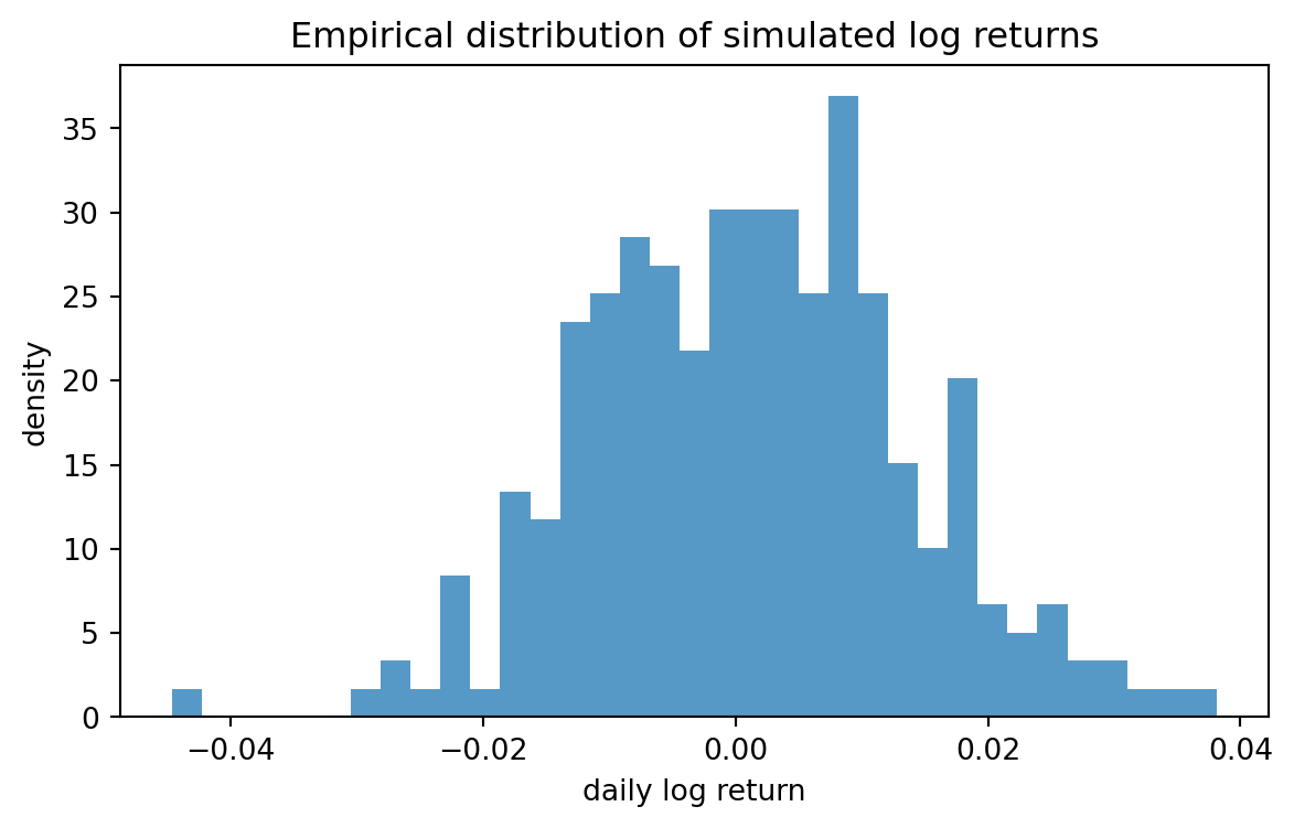
A basic empirical analysis of returns should include:
1. a time plot of returns;
2. a histogram or density estimate;
3. sample moments;
4. tail quantiles;
5. comparison with a fitted normal distribution;
6. checks for outliers and volatility clustering.
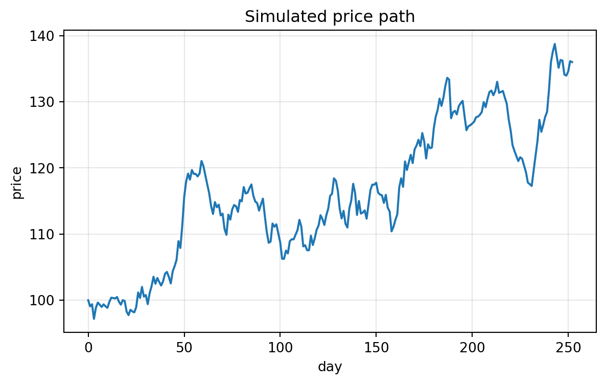
```{python}
#| label: ch07-empirical-returns-from-simulated-prices
#| fig-cap: "Computing simple and log returns from a simulated price series."
import numpy as np
import pandas as pd
import matplotlib.pyplot as plt

rng = np.random.default_rng(2026)
n_days = 252
S0 = 100.0
mu_daily = 0.0003
sigma_daily = 0.012

log_returns = rng.normal(mu_daily, sigma_daily, size=n_days)
prices = S0 * np.exp(np.cumsum(log_returns))
prices = np.insert(prices, 0, S0)

simple_returns = prices[1:] / prices[:-1] - 1
computed_log_returns = np.log(prices[1:] / prices[:-1])

returns_df = pd.DataFrame({
    "simple_return": simple_returns,
    "log_return": computed_log_returns
})

print(returns_df.describe())

plt.figure(figsize=(7, 4))
plt.plot(prices)
plt.xlabel("day")
plt.ylabel("price")
plt.title("Simulated price path")
plt.grid(True, alpha=0.3)
plt.show()

plt.figure(figsize=(7, 4))
plt.hist(computed_log_returns, bins=35, density=True, alpha=0.75)
plt.xlabel("daily log return")
plt.ylabel("density")
plt.title("Empirical distribution of simulated log returns")
plt.show()
```
## 7.14 QQ Plots and Distribution Diagnostics
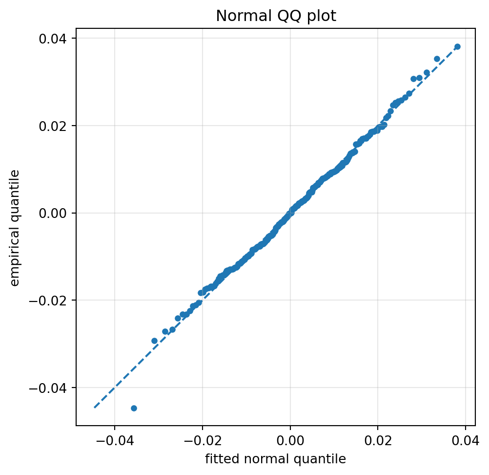
A QQ plot compares empirical quantiles with theoretical quantiles. If the return data are approximately normal, then a normal QQ plot should be close to a straight line.
For a sample
$$
x_1,\ldots,x_n,
$$
let
$$
x_{(1)}\le x_{(2)}\le\cdots\le x_{(n)}
$$
be the sorted sample. The empirical quantile $x_{(i)}$ is compared with a theoretical normal quantile
$$
\Phi^{-1}\left(\frac{i-1/2}{n}\right),
$$
where $\Phi$ is the standard normal cumulative distribution function.
Departures from a straight line in the tails suggest that the normal model may underestimate or overestimate extreme outcomes.
```{python}
#| label: ch07-qq-plot-with-normal-quantiles
#| fig-cap: "A normal QQ plot for simulated log returns."
import numpy as np
import matplotlib.pyplot as plt
from statistics import NormalDist

sample = computed_log_returns
n = len(sample)
sorted_sample = np.sort(sample)
probs = (np.arange(1, n + 1) - 0.5) / n
normal_quantiles = np.array([NormalDist().inv_cdf(p) for p in probs])

sample_mean = np.mean(sample)
sample_sd = np.std(sample, ddof=1)
fitted_quantiles = sample_mean + sample_sd * normal_quantiles

plt.figure(figsize=(5.5, 5.5))
plt.scatter(fitted_quantiles, sorted_sample, s=14)
lo = min(fitted_quantiles.min(), sorted_sample.min())
hi = max(fitted_quantiles.max(), sorted_sample.max())
plt.plot([lo, hi], [lo, hi], linestyle="--")
plt.xlabel("fitted normal quantile")
plt.ylabel("empirical quantile")
plt.title("Normal QQ plot")
plt.grid(True, alpha=0.3)
plt.show()
```
## 7.15 Annualization and Scaling Rules
Suppose daily log returns $X_1,\ldots,X_n$ are independent and identically distributed with
$$
\mathbb E[X_t]=\mu_d,
\qquad
\operatorname{Var}(X_t)=\sigma_d^2.
$$
The $n$-day cumulative log return is
$$
X_{1:n}=\sum_{t=1}^n X_t.
$$
Therefore
$$
\mathbb E[X_{1:n}]=n\mu_d,
\qquad
\operatorname{Var}(X_{1:n})=n\sigma_d^2.
$$
If there are about $252$ trading days per year, then
$$
\mu_{\mathrm{ann}}\approx 252\mu_d,
\qquad
\sigma_{\mathrm{ann}}\approx \sqrt{252}\sigma_d.
$$
The mean scales linearly in time. The standard deviation scales with the square root of time.
::: {.warning}
The annualization formula $\sigma_{\mathrm{ann}}=\sqrt{252}\sigma_d$ is not a law of nature. It follows from a model with uncorrelated returns and stable daily variance. If returns are dependent or volatility changes over time, this rule is only an approximation.
:::
## 7.16 Physical Probability versus Pricing Probability
In the previous chapters, the physical measure $\mathbb P$ described real-world probabilities, while the risk-neutral measure $\mathbb Q$ priced assets.
This distinction continues here.
Under the physical measure, a log return model might be
$$
X\sim N(\mu_P,\sigma^2).
$$
Under a risk-neutral measure, the drift changes to make discounted prices martingales. For example, if a one-period model has deterministic risk-free rate $r$, then risk-neutral pricing requires
$$
S_0=\frac{1}{1+r}\mathbb E^{\mathbb Q}[S_1].
$$
Equivalently,
$$
\mathbb E^{\mathbb Q}\left[\frac{S_1}{S_0}\right]=1+r.
$$
If $S_1=S_0e^X$ and $X\sim N(m_Q,v)$ under $\mathbb Q$, then
$$
\mathbb E^{\mathbb Q}\left[e^X\right]
=e^{m_Q+v/2}=1+r.
$$
Thus
$$
m_Q=\log(1+r)-\frac12v.
$$
This is an early appearance of a principle that will return in continuous time: risk-neutral modeling changes the drift, not necessarily the volatility.
## 7.17 AI Component: Reading Return Models Critically
::: {.ai-box}
### AI-assisted activity 7.1: Critique a return model
Ask an AI system to explain the statement:
> Daily log returns are normally distributed with constant mean and variance.
Then critique the response using the following checklist.
1. Did it distinguish log returns from simple returns?
2. Did it identify independence as a separate assumption?
3. Did it mention heavy tails and volatility clustering?
4. Did it explain why the model may still be useful as a first approximation?
5. Did it avoid saying that financial returns are exactly normal?
A high-quality explanation should be mathematically precise and empirically cautious.
:::
::: {.ai-box}
### AI-assisted activity 7.2: Formula audit
Give an AI system the following formulas and ask it to find any missing assumptions:
$$
\sigma_{\mathrm{ann}}=\sqrt{252}\sigma_{\mathrm{daily}},
$$
$$
\log\frac{S_n}{S_0}=\sum_{t=1}^n\log\frac{S_t}{S_{t-1}},
$$
$$
\mathbb E[S_T]=S_0e^{m+v/2}
\quad \text{if} \quad
\log(S_T/S_0)\sim N(m,v).
$$
The answer should state that the log-return identity is algebraic and requires positive prices, while the annualization rule and expectation formula require probabilistic assumptions.
:::
::: {.ai-box}
### AI-assisted activity 7.3: Code review prompt
Use the following prompt to review return-analysis code:
> Check this Python code for mathematical finance errors. Pay special attention to whether it confuses simple returns and log returns, annualizes volatility correctly, handles prices equal to zero, and uses sample variance with the correct degrees of freedom.
This prompt is useful because many coding errors in finance are not syntax errors. They are modeling errors.
:::
## 7.18 Python Mini-Lab: A Complete Return Analysis Workflow
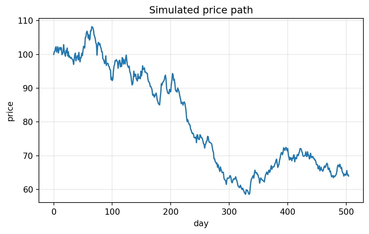
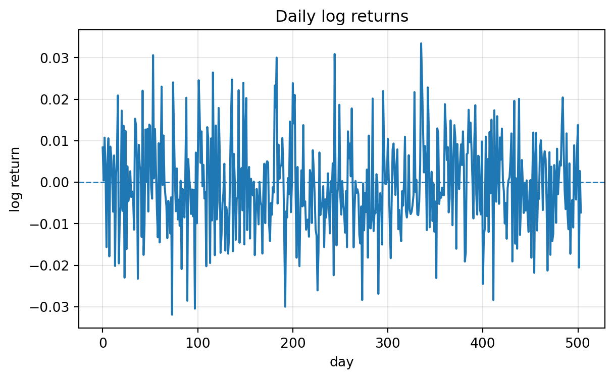
The following workflow combines the main ideas of the chapter using simulated prices. In a later lab, students can replace the simulated prices with historical data.
```{python}
#| label: ch07-return-analysis-workflow
#| fig-cap: "A compact return-analysis workflow."
import numpy as np
import pandas as pd
import matplotlib.pyplot as plt

rng = np.random.default_rng(5110)
n = 504
S0 = 100.0
mu_daily = 0.00025
sigma_daily = 0.011

# Simulate daily log returns and prices.
x = rng.normal(mu_daily, sigma_daily, size=n)
S = S0 * np.exp(np.cumsum(x))
S = np.insert(S, 0, S0)

# Compute returns from prices.
simple = S[1:] / S[:-1] - 1
logret = np.log(S[1:] / S[:-1])

# Summary statistics.
summary = {
    "mean daily log return": np.mean(logret),
    "daily volatility": np.std(logret, ddof=1),
    "annualized mean log return": 252 * np.mean(logret),
    "annualized volatility": np.sqrt(252) * np.std(logret, ddof=1),
    "lower 5 percent log-return quantile": np.quantile(logret, 0.05),
    "upper 95 percent log-return quantile": np.quantile(logret, 0.95),
    "minimum daily log return": np.min(logret),
    "maximum daily log return": np.max(logret)
}

pd.Series(summary)
```
```{python}
#| label: ch07-return-workflow-plots
#| fig-cap: "Price path and log-return path from the same simulated data."
plt.figure(figsize=(7, 4))
plt.plot(S)
plt.xlabel("day")
plt.ylabel("price")
plt.title("Simulated price path")
plt.grid(True, alpha=0.3)
plt.show()

plt.figure(figsize=(7, 4))
plt.plot(logret)
plt.axhline(0, linestyle="--", linewidth=1)
plt.xlabel("day")
plt.ylabel("log return")
plt.title("Daily log returns")
plt.grid(True, alpha=0.3)
plt.show()
```
## 7.19 Common Mistakes
1. **Confusing price levels with returns.** Prices are usually nonstationary; returns are often the modeled objects.
2. **Confusing simple and log returns.** Simple returns compound multiplicatively; log returns add over time.
3. **Assuming normality without checking tails.** Normal models are convenient, but empirical returns often have heavy tails.
4. **Interpreting volatility as total risk.** Volatility treats upside and downside deviations symmetrically.
5. **Annualizing without assumptions.** The square-root-of-time rule requires assumptions about dependence and variance.
6. **Using physical probabilities for pricing without justification.** Pricing usually uses a risk-neutral measure, not the historical probability measure.
7. **Ignoring data quality.** Missing prices, splits, dividends, and stale prices can distort returns.
## 7.20 Chapter Summary
This chapter introduced the probability language of financial returns.
The main ideas are:
- future returns are random variables;
- a distribution describes possible future outcomes and their probabilities;
- simple returns are natural for one-period percentage gains;
- log returns are additive over time;
- moments summarize center, dispersion, asymmetry, and tail thickness;
- covariance and correlation explain diversification;
- normal log returns imply lognormal prices;
- heavy tails are essential for risk modeling;
- empirical return analysis should check both central behavior and tail behavior;
- physical probabilities and pricing probabilities serve different roles.
The next chapter develops conditional expectation and information, which are needed for martingales, stochastic processes, and dynamic pricing.
## 7.21 Exercises
### Conceptual exercises
1. Explain why $S_{t+1}$ is modeled as a random variable at time $t$.
2. What is the difference between a simple return and a log return?
3. Why are log returns convenient for multi-period models?
4. Why does volatility not fully describe risk?
5. Explain why normal log returns imply positive prices.
6. What does it mean for returns to have heavy tails?
7. Explain why physical probability and risk-neutral probability should not be confused.
### Computational exercises
8. Suppose $S_0=50$, $S_1=55$, and $S_2=52$. Compute the one-period simple returns, one-period log returns, two-period simple return, and two-period log return.
9. A return $R$ takes values $-0.10$, $0.02$, and $0.15$ with probabilities $0.2$, $0.5$, and $0.3$. Compute $\mathbb E[R]$, $\operatorname{Var}(R)$, and $\sigma_R$.
10. Let $X\sim N(0.04,0.09)$. If $S_0=100$ and $S_T=S_0e^X$, compute $\mathbb E[S_T]$.
11. Suppose daily log-return volatility is $1.2\%$. Compute the annualized volatility using $252$ trading days. State the assumptions behind this calculation.
12. For two assets with volatilities $20\%$ and $30\%$, equal portfolio weights, and correlation $0.25$, compute portfolio volatility.
### Proof exercises
13. Prove that multi-period simple returns satisfy
$$
1+R_{0,n}=\prod_{t=1}^n(1+R_t).
$$
14. Prove that if $X\sim N(m,v)$, then $a+bX\sim N(a+bm,b^2v)$ for constants $a$ and $b$.
15. Prove that if $X_1$ and $X_2$ are independent normal random variables, then $X_1+X_2$ is normal. You may use moment generating functions.
16. Derive the two-asset portfolio variance formula.
### Python exercises
17. Write a Python function that takes a price vector and returns simple returns and log returns.
18. Simulate $10,000$ one-year terminal prices under normal log returns. Compare the empirical mean with $S_0e^{m+v/2}$.
19. Simulate normal and Student-t returns with the same approximate variance. Estimate the probability of a return more than three standard deviations from the mean.
20. Create a QQ plot for simulated Student-t returns against a fitted normal distribution. Explain what happens in the tails.
21. Estimate sample skewness and kurtosis for a simulated return series.
### AI-assisted exercises
22. Ask an AI system to explain why log returns add over time. Check whether it states the assumption $S_t>0$.
23. Ask an AI system to produce Python code for annualized volatility. Audit whether it uses standard deviation rather than variance.
24. Ask an AI system to compare normal and Student-t return models. Identify whether it explains the role of degrees of freedom.
25. Ask an AI system to interpret a histogram of returns. Revise the answer to include mathematical language about empirical distributions and tail probabilities.