21Chapter 18. Martingale Pricing in Continuous Time
21.1 Learning Goals
By the end of this chapter, students should be able to:
define discounted asset prices and self-financing wealth processes in continuous time;
explain why an equivalent martingale measure is the central mathematical object in no-arbitrage pricing;
prove the risk-neutral pricing formula for a replicable contingent claim;
distinguish physical probability, risk-neutral probability, and state-price density;
derive the Black–Scholes risk-neutral pricing formula from the martingale principle;
explain the relationship between completeness, martingale representation, and uniqueness of the martingale measure;
describe no-arbitrage price intervals in incomplete markets;
connect martingale pricing with stochastic discount factors and the Feynman–Kac PDE;
implement Monte Carlo risk-neutral pricing and check discounted martingale behavior in Python;
use AI tools to audit assumptions in continuous-time pricing arguments.
Continuous-time martingale pricing is the organizing principle behind modern derivative pricing.
A traded asset has a real-world statistical model under the physical measure \(\mathbb P\), but a derivative price is determined by no-arbitrage under a risk-neutral measure \(\mathbb Q\). Under \(\mathbb Q\), discounted traded asset prices are martingales:
The difference is that continuous time requires more care. Trading strategies must be adapted, stochastic integrals replace finite sums, and the absence of arbitrage is tied to semimartingale theory. In this book we use the clean diffusion setting needed for Black–Scholes-type models.
The main message is simple:
NoteMartingale pricing principle
After discounting by the money-market account, the price process of any traded asset should be a martingale under a risk-neutral measure.
This principle converts pricing into conditional expectation.
A strategy is self-financing if changes in wealth come only from gains and losses on existing holdings, not from adding or withdrawing cash. In differential form,
This formula is the continuous-time analogue of discounted gains from trade.
WarningWhy predictability matters
The holdings \(\phi_t\) must be chosen using information available before the infinitesimal price movement \(dS_t\) is realized. Otherwise the model would allow trading with knowledge of the future.
21.5 18.4 Admissible Strategies
Not every stochastic integral should be treated as a valid trading strategy. Without restrictions, continuous-time models can produce pathological doubling strategies.
A common admissibility condition is that discounted wealth is bounded from below:
\[
\widetilde V_t^\phi \ge -a
\qquad \text{for all }t\in[0,T]
\]
for some constant \(a\ge 0\).
This excludes strategies that finance possible arbitrage by allowing unlimited losses along the way.
For an introductory mathematical finance course, the important idea is:
NoteAdmissibility principle
A trading strategy must be adapted, self-financing, integrable with respect to asset prices, and economically reasonable enough to rule out infinite-loss schemes.
21.6 18.5 Equivalent Martingale Measures
A probability measure \(\mathbb Q\) is equivalent to \(\mathbb P\) if they agree on which events have probability zero:
The word equivalent preserves the same possible market scenarios. The word martingale gives the no-arbitrage pricing structure.
In a diffusion model, the equivalent martingale measure changes drift but preserves diffusion-driven randomness. For example, in the Black–Scholes model,
If \(\widetilde S\) is a \(\mathbb Q\)-martingale, then the stochastic integral is also a \(\mathbb Q\)-martingale under standard integrability assumptions. Hence
Therefore an equivalent martingale measure rules out arbitrage.
21.9 No-arbitrage implication
If there exists an equivalent martingale measure \(\mathbb Q\) under which discounted traded asset prices are martingales, then the model has no admissible arbitrage.
The converse is technically deeper in continuous time. The appropriate theorem uses the condition no free lunch with vanishing risk rather than only elementary arbitrage. In the diffusion models used in this book, the martingale-measure approach gives the correct no-arbitrage framework.
21.10 18.7 Pricing a Replicable Claim
Let \(X\) be a payoff at maturity \(T\). We say \(X\) is replicable if there exists a self-financing strategy \(\phi\) such that
\[
V_T^\phi=X.
\]
The no-arbitrage price of \(X\) at time \(t\) must be the wealth of the replicating strategy:
\[
V_t=V_t^\phi.
\]
Under an equivalent martingale measure \(\mathbb Q\), discounted wealth is a martingale. Therefore
Thus \(\widetilde S_t\) has zero drift under \(\mathbb Q\), so it is a martingale under suitable integrability conditions.
21.13 Interactive 18.1: Discounted stock price under \(\mathbb P\) and \(\mathbb Q\)
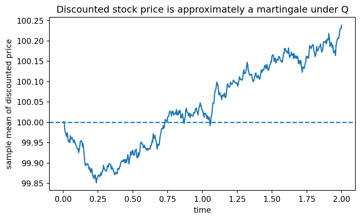
This demo compares the expected discounted stock price under two measures. Under the physical measure \(\mathbb P\), the drift is \(\mu\). Under the risk-neutral measure \(\mathbb Q\), the drift is \(r\).
If \(\mu\ne r\), then \(\mathbb E^{\mathbb P}[e^{-rt}S_t]\) is not constant. But under \(\mathbb Q\),
\[
\mathbb E^{\mathbb Q}[e^{-rt}S_t]=S_0.
\]
0.100
0.040
import numpy as npimport matplotlib.pyplot as pltrng = np.random.default_rng(7243)S0 =100.0r =0.04sigma =0.25T =2.0n_steps =252*2n_paths =50_000dt = T / n_stepsZ = rng.normal(size=(n_paths, n_steps))log_increments = (r -0.5* sigma**2) * dt + sigma * np.sqrt(dt) * Zlog_paths = np.cumsum(log_increments, axis=1)S = S0 * np.exp(log_paths)S = np.column_stack([np.full(n_paths, S0), S])times = np.linspace(0, T, n_steps +1)discounted_mean = np.exp(-r * times) * S.mean(axis=0)print("Initial stock price:", S0)print("Mean discounted price at T:", discounted_mean[-1])print("Monte Carlo error:", discounted_mean[-1] - S0)plt.figure(figsize=(7, 4))plt.plot(times, discounted_mean)plt.axhline(S0, linestyle="--")plt.xlabel("time")plt.ylabel("sample mean of discounted price")plt.title("Discounted stock price is approximately a martingale under Q")plt.show()
Initial stock price: 100.0
Mean discounted price at T: 100.23880077701288
Monte Carlo error: 0.2388007770128837
Monte Carlo check: discounted GBM is a martingale under the risk-neutral measure.
21.14 18.9 Risk-Neutral Pricing of a European Claim
Consider a European payoff
\[
X=g(S_T).
\]
If the short rate is constant and the market is complete, the time-\(t\) price is
For a call payoff \(g(S_T)=(S_T-K)^+\), this expectation gives the Black–Scholes formula. But the conditional-expectation viewpoint applies far more broadly.
Monte Carlo price: 8.372902728351082
Monte Carlo standard error: 0.020302718807799765
Black-Scholes price: 8.363276638981155
MC minus BS: 0.00962608936992737
21.15 18.10 Price Processes, Not Just Prices at Time Zero
The pricing formula defines an entire price process:
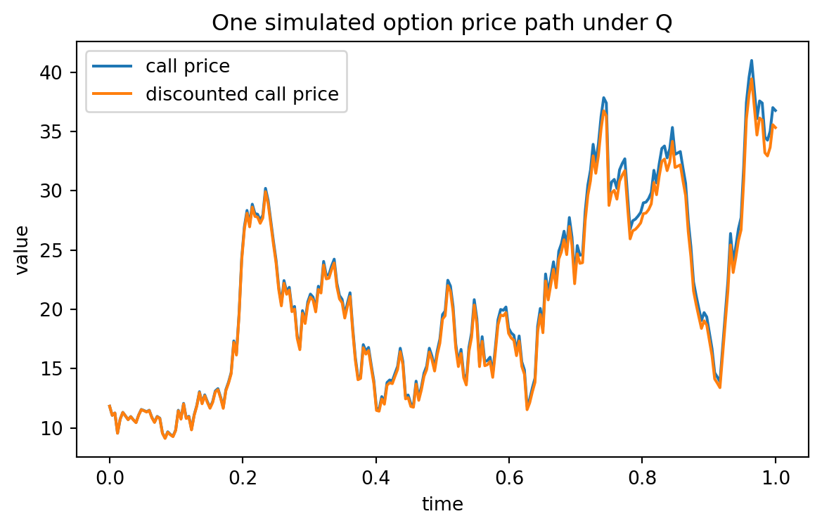
Thus the discounted derivative price is also a \(\mathbb Q\)-martingale.
21.16 Discounted derivative price martingale
If \(V_t\) is defined by risk-neutral valuation, then \(V_t/B_t\) is a \(\mathbb Q\)-martingale.
The martingale property is a consistency condition across time. If it failed, one could create dynamic arbitrage opportunities by buying or selling mispriced claims at different times.
21.17 18.11 Completeness and Uniqueness of the Martingale Measure
A market is complete if every reasonable contingent claim can be replicated by a self-financing trading strategy.
In continuous-time Brownian diffusion models, completeness is closely connected to the number of traded risky assets and the number of independent Brownian risk sources.
The market price of risk vector \(\lambda_t\in\mathbb R^m\) must satisfy
\[
\mu_t-r_t\mathbf 1=\Sigma_t\lambda_t.
\]
If this equation has a solution, an equivalent martingale measure can often be constructed. If the solution is unique and the model has enough tradable assets to span all Brownian risks, the market is complete.
A useful finite-dimensional intuition is:
if every source of randomness can be hedged by traded assets, the martingale measure is unique;
if some source of randomness cannot be traded, there are many martingale measures;
many martingale measures usually mean incomplete markets.
NoteComplete market principle
In a complete no-arbitrage market, every claim has exactly one no-arbitrage price because every claim can be replicated.
import numpy as npr =0.03mu = np.array([0.08, 0.06])Sigma = np.array([ [0.20, 0.10], [0.05, 0.18]])excess = mu - r * np.ones_like(mu)lambda_unique = np.linalg.solve(Sigma, excess)print("Volatility matrix Sigma:")print(Sigma)print("Excess drift vector:", excess)print("Market price of risk lambda:", lambda_unique)print("Check Sigma lambda:", Sigma @ lambda_unique)
A particular pricing model chooses one measure from this set using additional assumptions, such as utility preferences, calibration to market prices, or a model for volatility risk premium.
This is why the same payoff may have a unique Black–Scholes price in a complete idealized model, but require calibration choices in stochastic volatility, jump, or credit-risk models.
21.19 Interactive 18.2: Option price surface as a conditional expectation
A simulated Black-Scholes call price process and its discounted value.
21.20 18.13 Martingale Representation and Delta Hedging
In the one-dimensional Black–Scholes model, every square-integrable claim can be represented as a stochastic integral with respect to Brownian motion. Informally, for a discounted payoff \(X/B_T\), there exists an adapted process \(H_t\) such that
steps: 12 mean error: -0.00044 std error: 1.94836
steps: 52 mean error: 0.01356 std error: 0.94122
steps: 252 mean error: 0.00147 std error: 0.44287
21.21 18.14 Stochastic Discount Factors
Risk-neutral pricing can also be written using a stochastic discount factor, sometimes called a state-price density.
A positive random variable \(M_T\) is a stochastic discount factor if traded asset prices satisfy
\[
S_0^i=\mathbb E^{\mathbb P}[M_T S_T^i]
\]
for all traded assets \(i\).
If \(B_t=e^{rt}\) and \(Z_T=d\mathbb Q/d\mathbb P\), then
\[
M_T=e^{-rT}Z_T.
\]
For any payoff \(X\) priced by the same rule,
\[
V_0=\mathbb E^{\mathbb P}[M_T X].
\]
This form is useful because it expresses pricing under the physical measure \(\mathbb P\), but with a random discount factor that adjusts probabilities and time value simultaneously.
For Markov diffusion models, these are two forms of the same pricing principle.
import numpy as npfrom math import erf, sqrt, log, expK =100.0r =0.04sigma =0.25T =1.0def norm_cdf(x):return0.5* (1+ erf(x / sqrt(2)))def bs_call(S, t): tau = T - tif tau <=1e-12:returnmax(S - K, 0.0) d1 = (log(S / K) + (r +0.5* sigma**2) * tau) / (sigma * sqrt(tau)) d2 = d1 - sigma * sqrt(tau)return S * norm_cdf(d1) - K * exp(-r * tau) * norm_cdf(d2)S =105.0t =0.35hS =0.05ht =1e-4V = bs_call(S, t)Vt = (bs_call(S, t + ht) - bs_call(S, t - ht)) / (2* ht)VS = (bs_call(S + hS, t) - bs_call(S - hS, t)) / (2* hS)VSS = (bs_call(S + hS, t) -2* V + bs_call(S - hS, t)) / (hS**2)residual = Vt + r * S * VS +0.5* sigma**2* S**2* VSS - r * Vprint("PDE residual near zero:", residual)
PDE residual near zero: -2.0640680314931714e-06
21.23 18.16 Common Mistakes
Using the physical drift in pricing. The Black–Scholes price of a replicable claim does not use \(\mu\). It uses the risk-neutral drift \(r\).
Forgetting to discount. Martingales appear after discounting by \(B_t\). The stock price itself is generally not a martingale under \(\mathbb Q\) when \(r\ne0\).
Confusing expectation with prediction. The risk-neutral expectation is not a forecast of real-world average payoff. It is a no-arbitrage valuation rule.
Ignoring admissibility. Continuous-time trading rules require restrictions to rule out pathological arbitrage.
Assuming all markets are complete. Stochastic volatility, jumps, and credit-risk models are often incomplete. A martingale measure may not be unique.
Applying a formula outside its model. A closed-form Black–Scholes formula depends on constant volatility, continuous trading, no transaction costs, and complete-market assumptions.
21.24 18.17 AI-Assisted Learning Components
21.25 AI prompt: explain the pricing measure
Ask an AI tool:
Explain why the Black–Scholes option price does not depend on the physical drift \(\mu\). Use the words replication, discounting, martingale measure, and no-arbitrage. Then give a simple example of a wrong argument that incorrectly uses \(\mu\) in the option price.
Then check whether the response clearly separates statistical forecasting under \(\mathbb P\) from pricing under \(\mathbb Q\).
21.26 AI prompt: audit a proof
Give an AI tool the following claim:
Since \(S_t\) is a martingale under the risk-neutral measure, the discounted option price must equal \(\mathbb E^{\mathbb Q}[X\mid\mathcal F_t]\).
Ask it to find the mistake. A good answer should notice that \(S_t\) is generally not the martingale; \(S_t/B_t\) is. The correct price is
in the Black–Scholes model, changing from \(\mathbb P\) to \(\mathbb Q\) replaces \(\mu\) by \(r\);
completeness corresponds to the ability to replicate claims and is related to uniqueness of the equivalent martingale measure;
incomplete markets generally produce price intervals or require additional modeling assumptions;
martingale pricing and PDE pricing are connected through the Feynman–Kac formula.
The next chapter begins the study of fixed income, where the money-market account and discount factors become central objects rather than background notation.
21.29 18.19 Exercises
21.29.1 Conceptual Exercises
Explain why equivalent probability measures must agree on null events. Why is this important for financial modeling?
In your own words, distinguish the physical measure \(\mathbb P\) from the risk-neutral measure \(\mathbb Q\).
Why is it the discounted stock price, rather than the stock price itself, that should be a martingale under \(\mathbb Q\)?
Explain why a risk-neutral expectation is not the same as a real-world forecast.
What does it mean for a claim to be replicable? Why does replication imply a unique no-arbitrage price?
21.29.2 Mathematical Exercises
Suppose \(B_t=e^{rt}\) and \(S_t\) satisfies
\[
dS_t=rS_t\,dt+\sigma S_t\,dW_t^{\mathbb Q}.
\]
Use Itô’s formula to show that \(e^{-rt}S_t\) has zero drift.
Simulate risk-neutral GBM and verify that the sample average of \(e^{-rt}S_t\) is approximately constant over time.
Price a European put by Monte Carlo under \(\mathbb Q\) and compare the result with the Black–Scholes put formula.
Repeat the Monte Carlo option-pricing experiment using physical drift \(\mu\) instead of \(r\). Explain why the resulting number is not a no-arbitrage price.
Implement a function that estimates a call price and reports both the price and the Monte Carlo standard error.
Simulate discrete delta hedging errors for monthly, weekly, and daily rebalancing. Compare the standard deviation of the hedging error.
21.29.4 AI-Assisted Exercises
Ask an AI tool to explain why no-arbitrage pricing uses \(\mathbb Q\) rather than \(\mathbb P\). Identify one phrase in the response that is mathematically precise and one phrase that is potentially misleading.
Check whether it explicitly uses self-financing, discounting, and the martingale property.
Ask an AI tool to review your Monte Carlo code from Exercise 14. Record at least three concrete corrections or improvements.
Source Code
---title: "Chapter 18. Martingale Pricing in Continuous Time"---::: {.chapter-objectives}## Learning GoalsBy the end of this chapter, students should be able to:- define discounted asset prices and self-financing wealth processes in continuous time;- explain why an equivalent martingale measure is the central mathematical object in no-arbitrage pricing;- prove the risk-neutral pricing formula for a replicable contingent claim;- distinguish physical probability, risk-neutral probability, and state-price density;- derive the Black--Scholes risk-neutral pricing formula from the martingale principle;- explain the relationship between completeness, martingale representation, and uniqueness of the martingale measure;- describe no-arbitrage price intervals in incomplete markets;- connect martingale pricing with stochastic discount factors and the Feynman--Kac PDE;- implement Monte Carlo risk-neutral pricing and check discounted martingale behavior in Python;- use AI tools to audit assumptions in continuous-time pricing arguments.:::::: {.hero-box}Continuous-time martingale pricing is the organizing principle behind modern derivative pricing.A traded asset has a real-world statistical model under the physical measure $\mathbb P$, but a derivative price is determined by no-arbitrage under a risk-neutral measure $\mathbb Q$. Under $\mathbb Q$, discounted traded asset prices are martingales:$$\mathbb E^{\mathbb Q}\left[\frac{S_T}{B_T}\mid \mathcal F_t\right]=\frac{S_t}{B_t}.$$A replicable payoff $X$ has time-$t$ price$$V_t=B_t\mathbb E^{\mathbb Q}\left[\frac{X}{B_T}\mid\mathcal F_t\right].$$This formula is not a statistical forecasting formula. It is a no-arbitrage valuation formula.:::## 18.1 From Discrete-Time Pricing to Continuous-Time PricingIn discrete-time binomial models, we priced a payoff $X$ by backward induction or by risk-neutral expectation:$$V_n = B_n\mathbb E^{\mathbb Q}\left[\frac{X}{B_N}\mid\mathcal F_n\right].$$The continuous-time version has the same structure:$$V_t = B_t\mathbb E^{\mathbb Q}\left[\frac{X}{B_T}\mid\mathcal F_t\right],\qquad 0\le t\le T.$$The difference is that continuous time requires more care. Trading strategies must be adapted, stochastic integrals replace finite sums, and the absence of arbitrage is tied to semimartingale theory. In this book we use the clean diffusion setting needed for Black--Scholes-type models.The main message is simple:::: {.callout-note}## Martingale pricing principleAfter discounting by the money-market account, the price process of any traded asset should be a martingale under a risk-neutral measure.:::This principle converts pricing into conditional expectation.## 18.2 The Continuous-Time Market ModelWork on a filtered probability space$$(\Omega,\mathcal F,(\mathcal F_t)_{0\le t\le T},\mathbb P),$$where $\mathcal F_t$ represents all information available by time $t$.The money-market account is denoted by $B_t$. If the short rate is deterministic or adapted and integrable, then$$dB_t=r_tB_t\,dt,\qquad B_0=1,$$so$$B_t=\exp\left(\int_0^t r_s\,ds\right).$$For constant $r$,$$B_t=e^{rt}.$$Let $S_t=(S_t^1,\ldots,S_t^d)^\top$ be the vector of risky asset prices. The discounted prices are$$\widetilde S_t^i=\frac{S_t^i}{B_t},\qquad i=1,\ldots,d.$$In vector form,$$\widetilde S_t = B_t^{-1}S_t.$$Discounting places all cash flows in the same time units. A dollar tomorrow is not the same object as a dollar today unless it is discounted.## 18.3 Trading Strategies and WealthA trading strategy is a predictable process$$\phi_t=(\phi_t^0,\phi_t^1,\ldots,\phi_t^d),$$where $\phi_t^0$ is the number of units held in the money-market account and $\phi_t^i$ is the number of shares held in asset $i$.The wealth process is$$V_t^\phi = \phi_t^0B_t+\sum_{i=1}^d\phi_t^iS_t^i.$$A strategy is **self-financing** if changes in wealth come only from gains and losses on existing holdings, not from adding or withdrawing cash. In differential form,$$dV_t^\phi=\phi_t^0\,dB_t+\sum_{i=1}^d\phi_t^i\,dS_t^i.$$For discounted wealth,$$\widetilde V_t^\phi=\frac{V_t^\phi}{B_t},$$the self-financing condition becomes$$d\widetilde V_t^\phi=\sum_{i=1}^d\phi_t^i\,d\widetilde S_t^i.$$Equivalently,$$\widetilde V_t^\phi=\widetilde V_0^\phi+\int_0^t \phi_s^\top\,d\widetilde S_s.$$This formula is the continuous-time analogue of discounted gains from trade.::: {.callout-warning}## Why predictability mattersThe holdings $\phi_t$ must be chosen using information available before the infinitesimal price movement $dS_t$ is realized. Otherwise the model would allow trading with knowledge of the future.:::## 18.4 Admissible StrategiesNot every stochastic integral should be treated as a valid trading strategy. Without restrictions, continuous-time models can produce pathological doubling strategies.A common admissibility condition is that discounted wealth is bounded from below:$$\widetilde V_t^\phi \ge -a\qquad \text{for all }t\in[0,T]$$for some constant $a\ge 0$.This excludes strategies that finance possible arbitrage by allowing unlimited losses along the way.For an introductory mathematical finance course, the important idea is:::: {.callout-note}## Admissibility principleA trading strategy must be adapted, self-financing, integrable with respect to asset prices, and economically reasonable enough to rule out infinite-loss schemes.:::## 18.5 Equivalent Martingale MeasuresA probability measure $\mathbb Q$ is equivalent to $\mathbb P$ if they agree on which events have probability zero:$$\mathbb Q(A)=0\quad \Longleftrightarrow \quad\mathbb P(A)=0.$$This means $\mathbb Q$ does not remove or add possible paths. It only changes their probabilities.::: {.definition}## Equivalent martingale measureA probability measure $\mathbb Q$ is an **equivalent martingale measure** for the market if:1. $\mathbb Q$ is equivalent to $\mathbb P$;2. each discounted risky asset price $\widetilde S^i_t=S_t^i/B_t$ is a martingale under $\mathbb Q$.That is,$$\mathbb E^{\mathbb Q}[\widetilde S_t^i\mid\mathcal F_s]=\widetilde S_s^i,\qquad 0\le s\le t\le T.$$:::The word **equivalent** preserves the same possible market scenarios. The word **martingale** gives the no-arbitrage pricing structure.In a diffusion model, the equivalent martingale measure changes drift but preserves diffusion-driven randomness. For example, in the Black--Scholes model,$$dS_t=\mu S_t\,dt+\sigma S_t\,dW_t^{\mathbb P}$$under $\mathbb P$, while under $\mathbb Q$,$$dS_t=rS_t\,dt+\sigma S_t\,dW_t^{\mathbb Q}.$$The volatility $\sigma$ is unchanged; the drift becomes $r$.## 18.6 Why Martingale Measures Rule Out ArbitrageSuppose $\mathbb Q$ is an equivalent martingale measure and $\phi$ is a self-financing admissible strategy. Then discounted wealth satisfies$$\widetilde V_t^\phi=\widetilde V_0^\phi+\int_0^t \phi_s^\top\,d\widetilde S_s.$$If $\widetilde S$ is a $\mathbb Q$-martingale, then the stochastic integral is also a $\mathbb Q$-martingale under standard integrability assumptions. Hence$$\mathbb E^{\mathbb Q}[\widetilde V_T^\phi]=\widetilde V_0^\phi.$$Now suppose an arbitrage starts with zero wealth and ends with nonnegative wealth, with positive probability of strictly positive wealth:$$\widetilde V_0^\phi=0,\qquad\widetilde V_T^\phi\ge 0,\qquad\mathbb Q(\widetilde V_T^\phi>0)>0.$$Then$$\mathbb E^{\mathbb Q}[\widetilde V_T^\phi]>0,$$which contradicts$$\mathbb E^{\mathbb Q}[\widetilde V_T^\phi]=\widetilde V_0^\phi=0.$$Therefore an equivalent martingale measure rules out arbitrage.::: {.theorem}## No-arbitrage implicationIf there exists an equivalent martingale measure $\mathbb Q$ under which discounted traded asset prices are martingales, then the model has no admissible arbitrage.:::The converse is technically deeper in continuous time. The appropriate theorem uses the condition **no free lunch with vanishing risk** rather than only elementary arbitrage. In the diffusion models used in this book, the martingale-measure approach gives the correct no-arbitrage framework.## 18.7 Pricing a Replicable ClaimLet $X$ be a payoff at maturity $T$. We say $X$ is **replicable** if there exists a self-financing strategy $\phi$ such that$$V_T^\phi=X.$$The no-arbitrage price of $X$ at time $t$ must be the wealth of the replicating strategy:$$V_t=V_t^\phi.$$Under an equivalent martingale measure $\mathbb Q$, discounted wealth is a martingale. Therefore$$\frac{V_t}{B_t}=\mathbb E^{\mathbb Q}\left[\frac{V_T}{B_T}\mid\mathcal F_t\right]=\mathbb E^{\mathbb Q}\left[\frac{X}{B_T}\mid\mathcal F_t\right].$$Multiplying by $B_t$ gives the central formula:::: {.theorem}## Risk-neutral pricing formula for a replicable claimIf $X$ is a replicable payoff at time $T$, and $\mathbb Q$ is an equivalent martingale measure, then its no-arbitrage price at time $t$ is$$V_t=B_t\mathbb E^{\mathbb Q}\left[\frac{X}{B_T}\mid\mathcal F_t\right].$$If $r$ is constant, then$$V_t=e^{-r(T-t)}\mathbb E^{\mathbb Q}[X\mid\mathcal F_t].$$:::This formula is valid for any replicable claim, not only vanilla options.## 18.8 Discounted Prices as Martingales: A Black--Scholes CheckUnder the risk-neutral Black--Scholes model,$$dS_t=rS_t\,dt+\sigma S_t\,dW_t^{\mathbb Q}.$$The discounted stock price is$$\widetilde S_t=e^{-rt}S_t.$$Using Itô's product rule,$$d\widetilde S_t=e^{-rt}\,dS_t-r e^{-rt}S_t\,dt.$$Substitute the risk-neutral dynamics:$$d\widetilde S_t=e^{-rt}(rS_t\,dt+\sigma S_t\,dW_t^{\mathbb Q})-r e^{-rt}S_t\,dt.$$The drift terms cancel:$$d\widetilde S_t=\sigma\widetilde S_t\,dW_t^{\mathbb Q}.$$Thus $\widetilde S_t$ has zero drift under $\mathbb Q$, so it is a martingale under suitable integrability conditions.::: {.interactive-card}## Interactive 18.1: Discounted stock price under $\mathbb P$ and $\mathbb Q$This demo compares the expected discounted stock price under two measures. Under the physical measure $\mathbb P$, the drift is $\mu$. Under the risk-neutral measure $\mathbb Q$, the drift is $r$.If $\mu\ne r$, then $\mathbb E^{\mathbb P}[e^{-rt}S_t]$ is not constant. But under $\mathbb Q$,$$\mathbb E^{\mathbb Q}[e^{-rt}S_t]=S_0.$$<div class="mf-control-row"><label for="ch18-mu-slider">Physical drift $\mu$:</label><input id="ch18-mu-slider" type="range" min="-0.05" max="0.20" step="0.005" value="0.10"><span id="ch18-mu-value" class="mf-badge">0.100</span></div><div class="mf-control-row"><label for="ch18-r-slider">Rate $r$:</label><input id="ch18-r-slider" type="range" min="0.00" max="0.10" step="0.005" value="0.04"><span id="ch18-r-value" class="mf-badge">0.040</span></div><div id="ch18-discounted-demo" class="plotly-demo"></div>:::<script>window.mfPlotlyReady(function() {var el =document.getElementById("ch18-discounted-demo");var muSlider =document.getElementById("ch18-mu-slider");var rSlider =document.getElementById("ch18-r-slider");var muLabel =document.getElementById("ch18-mu-value");var rLabel =document.getElementById("ch18-r-value");if (!el ||!muSlider ||!rSlider ||!muLabel ||!rLabel) return;var S0 =100;var times = [];for (var i =0; i <=200; i++) times.push(2* i /200);functiondraw() {var mu =parseFloat(muSlider.value);var r =parseFloat(rSlider.value); muLabel.textContent= mu.toFixed(3); rLabel.textContent= r.toFixed(3);var underP = times.map(function(t) { return S0 *Math.exp((mu - r) * t); });var underQ = times.map(function(t) { return S0; });var traces = [ {x: times,y: underP,mode:"lines",name:"E_P[exp(-rt) S_t]"}, {x: times,y: underQ,mode:"lines",name:"E_Q[exp(-rt) S_t]"} ];var layout = {title:"Expected Discounted Stock Price",xaxis: {title:"time t"},yaxis: {title:"expected discounted price"},margin: {l:70,r:20,t:55,b:55},legend: {orientation:"h"} }; Plotly.react(el, traces, layout, {responsive:true}); } muSlider.addEventListener("input", draw); rSlider.addEventListener("input", draw);draw();});</script>```{python}#| label: py-ch18-discounted-gbm-martingale#| fig-cap: "Monte Carlo check: discounted GBM is a martingale under the risk-neutral measure."import numpy as npimport matplotlib.pyplot as pltrng = np.random.default_rng(7243)S0 =100.0r =0.04sigma =0.25T =2.0n_steps =252*2n_paths =50_000dt = T / n_stepsZ = rng.normal(size=(n_paths, n_steps))log_increments = (r -0.5* sigma**2) * dt + sigma * np.sqrt(dt) * Zlog_paths = np.cumsum(log_increments, axis=1)S = S0 * np.exp(log_paths)S = np.column_stack([np.full(n_paths, S0), S])times = np.linspace(0, T, n_steps +1)discounted_mean = np.exp(-r * times) * S.mean(axis=0)print("Initial stock price:", S0)print("Mean discounted price at T:", discounted_mean[-1])print("Monte Carlo error:", discounted_mean[-1] - S0)plt.figure(figsize=(7, 4))plt.plot(times, discounted_mean)plt.axhline(S0, linestyle="--")plt.xlabel("time")plt.ylabel("sample mean of discounted price")plt.title("Discounted stock price is approximately a martingale under Q")plt.show()```## 18.9 Risk-Neutral Pricing of a European ClaimConsider a European payoff$$X=g(S_T).$$If the short rate is constant and the market is complete, the time-$t$ price is$$V_t=e^{-r(T-t)}\mathbb E^{\mathbb Q}[g(S_T)\mid\mathcal F_t].$$In the Black--Scholes model, $S_T$ conditional on $\mathcal F_t$ is lognormal:$$S_T=S_t\exp\left(\left(r-\frac12\sigma^2\right)(T-t)+\sigma(W_T^{\mathbb Q}-W_t^{\mathbb Q})\right).$$Thus$$V(t,S_t)=e^{-r(T-t)}\mathbb E^{\mathbb Q}\left[g\left(S_t e^{(r-\frac12\sigma^2)(T-t)+\sigma\sqrt{T-t}Z}\right)\right],$$where $Z\sim N(0,1)$.For a call payoff $g(S_T)=(S_T-K)^+$, this expectation gives the Black--Scholes formula. But the conditional-expectation viewpoint applies far more broadly.```{python}#| label: py-ch18-monte-carlo-call-pricing#| fig-cap: "Risk-neutral Monte Carlo pricing for a European call."import numpy as npfrom math import erf, sqrt, log, exprng = np.random.default_rng(5110)S0 =100.0K =105.0r =0.04sigma =0.22T =1.0n =500_000Z = rng.normal(size=n)ST = S0 * np.exp((r -0.5* sigma**2) * T + sigma * np.sqrt(T) * Z)payoff = np.maximum(ST - K, 0.0)mc_price = np.exp(-r * T) * np.mean(payoff)mc_se = np.exp(-r * T) * np.std(payoff, ddof=1) / np.sqrt(n)def norm_cdf(x):return0.5* (1.0+ erf(x / sqrt(2.0)))d1 = (log(S0 / K) + (r +0.5* sigma**2) * T) / (sigma * sqrt(T))d2 = d1 - sigma * sqrt(T)bs_price = S0 * norm_cdf(d1) - K * exp(-r * T) * norm_cdf(d2)print("Monte Carlo price:", mc_price)print("Monte Carlo standard error:", mc_se)print("Black-Scholes price:", bs_price)print("MC minus BS:", mc_price - bs_price)```## 18.10 Price Processes, Not Just Prices at Time ZeroThe pricing formula defines an entire price process:$$V_t=B_t\mathbb E^{\mathbb Q}\left[\frac{X}{B_T}\mid\mathcal F_t\right].$$Therefore the discounted derivative price is$$\widetilde V_t=\frac{V_t}{B_t}=\mathbb E^{\mathbb Q}\left[\frac{X}{B_T}\mid\mathcal F_t\right].$$By the tower property,$$\mathbb E^{\mathbb Q}[\widetilde V_t\mid\mathcal F_s]=\widetilde V_s,\qquad 0\le s\le t\le T.$$Thus the discounted derivative price is also a $\mathbb Q$-martingale.::: {.theorem}## Discounted derivative price martingaleIf $V_t$ is defined by risk-neutral valuation, then $V_t/B_t$ is a $\mathbb Q$-martingale.:::The martingale property is a consistency condition across time. If it failed, one could create dynamic arbitrage opportunities by buying or selling mispriced claims at different times.## 18.11 Completeness and Uniqueness of the Martingale MeasureA market is complete if every reasonable contingent claim can be replicated by a self-financing trading strategy.In continuous-time Brownian diffusion models, completeness is closely connected to the number of traded risky assets and the number of independent Brownian risk sources.For example, suppose$$dS_t^i=S_t^i\left(\mu_i\,dt+\sum_{j=1}^m\sigma_{ij}\,dW_t^j\right),\qquad i=1,\ldots,d.$$The volatility matrix is$$\Sigma=(\sigma_{ij})_{d\times m}.$$The market price of risk vector $\lambda_t\in\mathbb R^m$ must satisfy$$\mu_t-r_t\mathbf 1=\Sigma_t\lambda_t.$$If this equation has a solution, an equivalent martingale measure can often be constructed. If the solution is unique and the model has enough tradable assets to span all Brownian risks, the market is complete.A useful finite-dimensional intuition is:- if every source of randomness can be hedged by traded assets, the martingale measure is unique;- if some source of randomness cannot be traded, there are many martingale measures;- many martingale measures usually mean incomplete markets.::: {.callout-note}## Complete market principleIn a complete no-arbitrage market, every claim has exactly one no-arbitrage price because every claim can be replicated.:::```{python}#| label: py-ch18-market-price-risk-linear-system#| fig-cap: "Solving the market price of risk equation in a multi-asset diffusion model."import numpy as npr =0.03mu = np.array([0.08, 0.06])Sigma = np.array([ [0.20, 0.10], [0.05, 0.18]])excess = mu - r * np.ones_like(mu)lambda_unique = np.linalg.solve(Sigma, excess)print("Volatility matrix Sigma:")print(Sigma)print("Excess drift vector:", excess)print("Market price of risk lambda:", lambda_unique)print("Check Sigma lambda:", Sigma @ lambda_unique)```## 18.12 Incomplete Markets and Price IntervalsIn an incomplete market, not every payoff is replicable. Then martingale pricing may not produce a unique price.Let $\mathcal M$ be the set of equivalent martingale measures. For a nonreplicable payoff $X$, no-arbitrage usually gives a price interval:$$\inf_{\mathbb Q\in\mathcal M}B_t\mathbb E^{\mathbb Q}\left[\frac{X}{B_T}\mid\mathcal F_t\right]\le V_t\le\sup_{\mathbb Q\in\mathcal M}B_t\mathbb E^{\mathbb Q}\left[\frac{X}{B_T}\mid\mathcal F_t\right].$$A particular pricing model chooses one measure from this set using additional assumptions, such as utility preferences, calibration to market prices, or a model for volatility risk premium.This is why the same payoff may have a unique Black--Scholes price in a complete idealized model, but require calibration choices in stochastic volatility, jump, or credit-risk models.::: {.interactive-card}## Interactive 18.2: Option price surface as a conditional expectationFor a European call, the risk-neutral price is$$C(t,S)=e^{-r(T-t)}\mathbb E^{\mathbb Q}[(S_T-K)^+\mid S_t=S].$$Use the slider to change the time $t$. As $t$ approaches maturity $T$, the smooth price curve approaches the kinked payoff $(S-K)^+$.<div class="mf-control-row"><label for="ch18-time-slider">Current time $t$:</label><input id="ch18-time-slider" type="range" min="0" max="0.99" step="0.01" value="0.25"><span id="ch18-time-value" class="mf-badge">0.25</span></div><div id="ch18-call-curve-demo" class="plotly-demo"></div>:::<script>window.mfPlotlyReady(function() {var el =document.getElementById("ch18-call-curve-demo");var slider =document.getElementById("ch18-time-slider");var label =document.getElementById("ch18-time-value");if (!el ||!slider ||!label) return;var K =100;var r =0.04;var sigma =0.25;var T =1.0;functionerfApprox(x) {var sign = x >=0?1:-1; x =Math.abs(x);var a1 =0.254829592;var a2 =-0.284496736;var a3 =1.421413741;var a4 =-1.453152027;var a5 =1.061405429;var p =0.3275911;var t =1.0/ (1.0+ p * x);var y =1.0- (((((a5 * t + a4) * t) + a3) * t + a2) * t + a1) * t *Math.exp(-x * x);return sign * y; }functionnormCdf(x) {return0.5* (1+erfApprox(x /Math.sqrt(2))); }functioncallPrice(S, tau) {if (tau <=1e-8) returnMath.max(S - K,0);var d1 = (Math.log(S / K) + (r +0.5* sigma * sigma) * tau) / (sigma *Math.sqrt(tau));var d2 = d1 - sigma *Math.sqrt(tau);return S *normCdf(d1) - K *Math.exp(-r * tau) *normCdf(d2); }var Sgrid = [];for (var i =0; i <=240; i++) Sgrid.push(40+140* i /240);functiondraw() {var t =parseFloat(slider.value); label.textContent= t.toFixed(2);var tau =Math.max(T - t,1e-8);var prices = Sgrid.map(function(S) { returncallPrice(S, tau); });var payoff = Sgrid.map(function(S) { returnMath.max(S - K,0); });var traces = [ {x: Sgrid,y: prices,mode:"lines",name:"call price C(t,S)"}, {x: Sgrid,y: payoff,mode:"lines",name:"payoff at maturity"} ];var layout = {title:"Risk-Neutral Call Price Curve",xaxis: {title:"stock price S"},yaxis: {title:"value"},margin: {l:60,r:20,t:55,b:55},legend: {orientation:"h"} }; Plotly.react(el, traces, layout, {responsive:true}); } slider.addEventListener("input", draw);draw();});</script>```{python}#| label: py-ch18-price-process-simulation#| fig-cap: "A simulated Black-Scholes call price process and its discounted value."import numpy as npimport matplotlib.pyplot as pltfrom math import erf, sqrt, log, exprng = np.random.default_rng(2026)S0 =100.0K =100.0r =0.04sigma =0.25T =1.0n_steps =252def norm_cdf(x):return0.5* (1+ erf(x / sqrt(2)))def bs_call(S, K, r, sigma, tau):if tau <=1e-12:returnmax(S - K, 0.0) d1 = (log(S / K) + (r +0.5* sigma**2) * tau) / (sigma * sqrt(tau)) d2 = d1 - sigma * sqrt(tau)return S * norm_cdf(d1) - K * exp(-r * tau) * norm_cdf(d2)dt = T / n_stepstimes = np.linspace(0, T, n_steps +1)Z = rng.normal(size=n_steps)log_returns = (r -0.5* sigma**2) * dt + sigma * sqrt(dt) * ZS_path = np.r_[S0, S0 * np.exp(np.cumsum(log_returns))]C_path = np.array([bs_call(S_path[i], K, r, sigma, T - times[i]) for i inrange(n_steps +1)])disc_C = np.exp(-r * times) * C_pathplt.figure(figsize=(7, 4))plt.plot(times, C_path, label="call price")plt.plot(times, disc_C, label="discounted call price")plt.xlabel("time")plt.ylabel("value")plt.title("One simulated option price path under Q")plt.legend()plt.show()```## 18.13 Martingale Representation and Delta HedgingIn the one-dimensional Black--Scholes model, every square-integrable claim can be represented as a stochastic integral with respect to Brownian motion. Informally, for a discounted payoff $X/B_T$, there exists an adapted process $H_t$ such that$$\frac{X}{B_T}=\mathbb E^{\mathbb Q}\left[\frac{X}{B_T}\right]+\int_0^T H_t\,dW_t^{\mathbb Q}.$$Because the discounted stock satisfies$$d\widetilde S_t=\sigma\widetilde S_t\,dW_t^{\mathbb Q},$$we can rewrite the representation as an integral with respect to $\widetilde S_t$:$$\frac{X}{B_T}=V_0+\int_0^T \Delta_t\,d\widetilde S_t.$$The process $\Delta_t$ is the number of shares in the stock. In the Black--Scholes PDE approach,$$\Delta_t=\frac{\partial V}{\partial S}(t,S_t).$$This is the mathematical reason delta hedging replicates the option.```{python}#| label: py-ch18-discrete-delta-hedging#| fig-cap: "Discrete delta hedging error decreases as rebalancing becomes more frequent."import numpy as npfrom math import erf, sqrt, log, exprng = np.random.default_rng(7339)S0 =100.0K =100.0r =0.03sigma =0.20T =1.0n_paths =5000def norm_cdf(x):return0.5* (1+ erf(x / sqrt(2)))def bs_call_delta(S, K, r, sigma, tau):if tau <=1e-12:return1.0if S > K else0.0 d1 = (log(S / K) + (r +0.5* sigma**2) * tau) / (sigma * sqrt(tau))return norm_cdf(d1)def bs_call(S, K, r, sigma, tau):if tau <=1e-12:returnmax(S - K, 0.0) d1 = (log(S / K) + (r +0.5* sigma**2) * tau) / (sigma * sqrt(tau)) d2 = d1 - sigma * sqrt(tau)return S * norm_cdf(d1) - K * exp(-r * tau) * norm_cdf(d2)def hedge_errors(n_steps): dt = T / n_steps errors = []for _ inrange(n_paths): S = S0 option_value = bs_call(S, K, r, sigma, T) delta = bs_call_delta(S, K, r, sigma, T) cash = option_value - delta * Sfor j inrange(n_steps): tau_next = T - (j +1) * dt z = rng.normal() S_next = S * exp((r -0.5* sigma**2) * dt + sigma * sqrt(dt) * z) cash *= exp(r * dt) new_delta = bs_call_delta(S_next, K, r, sigma, tau_next) cash -= (new_delta - delta) * S_next S = S_next delta = new_delta portfolio = delta * S + cash payoff =max(S - K, 0.0) errors.append(portfolio - payoff)return np.array(errors)for n_steps in [12, 52, 252]: err = hedge_errors(n_steps)print("steps:", n_steps,"mean error:", round(err.mean(), 5),"std error:", round(err.std(ddof=1), 5))```## 18.14 Stochastic Discount FactorsRisk-neutral pricing can also be written using a stochastic discount factor, sometimes called a state-price density.A positive random variable $M_T$ is a stochastic discount factor if traded asset prices satisfy$$S_0^i=\mathbb E^{\mathbb P}[M_T S_T^i]$$for all traded assets $i$.If $B_t=e^{rt}$ and $Z_T=d\mathbb Q/d\mathbb P$, then$$M_T=e^{-rT}Z_T.$$For any payoff $X$ priced by the same rule,$$V_0=\mathbb E^{\mathbb P}[M_T X].$$This form is useful because it expresses pricing under the physical measure $\mathbb P$, but with a random discount factor that adjusts probabilities and time value simultaneously.The connection is direct:$$\mathbb E^{\mathbb P}[M_T X]=e^{-rT}\mathbb E^{\mathbb P}[Z_T X]=e^{-rT}\mathbb E^{\mathbb Q}[X].$$```{python}#| label: py-ch18-stochastic-discount-factor#| fig-cap: "Pricing with a stochastic discount factor equals risk-neutral pricing."import numpy as nprng = np.random.default_rng(31415)S0 =100.0K =100.0mu =0.09r =0.03sigma =0.20T =1.0n =400_000Zp = rng.normal(size=n)WT = np.sqrt(T) * ZpST_P = S0 * np.exp((mu -0.5* sigma**2) * T + sigma * WT)lambda_mpr = (mu - r) / sigmaZ_density = np.exp(-lambda_mpr * WT -0.5* lambda_mpr**2* T)M = np.exp(-r * T) * Z_densitypayoff = np.maximum(ST_P - K, 0.0)price_sdf = np.mean(M * payoff)stock_check = np.mean(M * ST_P)bond_check = np.mean(M * np.exp(r * T))print("Call price from stochastic discount factor:", price_sdf)print("Check stock price E_P[M S_T]:", stock_check)print("Check bond price E_P[M B_T]:", bond_check)```## 18.15 Martingale Pricing and the Feynman--Kac FormulaSuppose a Markov state process has risk-neutral dynamics$$dS_t=rS_t\,dt+\sigma S_t\,dW_t^{\mathbb Q}.$$Let$$V(t,S)=e^{-r(T-t)}\mathbb E^{\mathbb Q}[g(S_T)\mid S_t=S].$$Then $V$ solves the Black--Scholes PDE:$$V_t+rS V_S+\frac12\sigma^2S^2V_{SS}-rV=0,$$with terminal condition$$V(T,S)=g(S).$$This is an instance of the Feynman--Kac formula. It connects conditional expectations to PDEs.::: {.callout-note}## Two equivalent viewsThe martingale view says:$$V_t=e^{-r(T-t)}\mathbb E^{\mathbb Q}[g(S_T)\mid\mathcal F_t].$$The PDE view says:$$V_t+rS V_S+\frac12\sigma^2S^2V_{SS}-rV=0.$$For Markov diffusion models, these are two forms of the same pricing principle.:::```{python}#| label: py-ch18-pde-residual-check#| fig-cap: "Numerical check of the Black-Scholes PDE residual using finite differences."import numpy as npfrom math import erf, sqrt, log, expK =100.0r =0.04sigma =0.25T =1.0def norm_cdf(x):return0.5* (1+ erf(x / sqrt(2)))def bs_call(S, t): tau = T - tif tau <=1e-12:returnmax(S - K, 0.0) d1 = (log(S / K) + (r +0.5* sigma**2) * tau) / (sigma * sqrt(tau)) d2 = d1 - sigma * sqrt(tau)return S * norm_cdf(d1) - K * exp(-r * tau) * norm_cdf(d2)S =105.0t =0.35hS =0.05ht =1e-4V = bs_call(S, t)Vt = (bs_call(S, t + ht) - bs_call(S, t - ht)) / (2* ht)VS = (bs_call(S + hS, t) - bs_call(S - hS, t)) / (2* hS)VSS = (bs_call(S + hS, t) -2* V + bs_call(S - hS, t)) / (hS**2)residual = Vt + r * S * VS +0.5* sigma**2* S**2* VSS - r * Vprint("PDE residual near zero:", residual)```## 18.16 Common Mistakes1. **Using the physical drift in pricing.** The Black--Scholes price of a replicable claim does not use $\mu$. It uses the risk-neutral drift $r$.2. **Forgetting to discount.** Martingales appear after discounting by $B_t$. The stock price itself is generally not a martingale under $\mathbb Q$ when $r\ne0$.3. **Confusing expectation with prediction.** The risk-neutral expectation is not a forecast of real-world average payoff. It is a no-arbitrage valuation rule.4. **Ignoring admissibility.** Continuous-time trading rules require restrictions to rule out pathological arbitrage.5. **Assuming all markets are complete.** Stochastic volatility, jumps, and credit-risk models are often incomplete. A martingale measure may not be unique.6. **Applying a formula outside its model.** A closed-form Black--Scholes formula depends on constant volatility, continuous trading, no transaction costs, and complete-market assumptions.## 18.17 AI-Assisted Learning Components::: {.ai-box}## AI prompt: explain the pricing measureAsk an AI tool:> Explain why the Black--Scholes option price does not depend on the physical drift $\mu$. Use the words replication, discounting, martingale measure, and no-arbitrage. Then give a simple example of a wrong argument that incorrectly uses $\mu$ in the option price.Then check whether the response clearly separates statistical forecasting under $\mathbb P$ from pricing under $\mathbb Q$.:::::: {.ai-box}## AI prompt: audit a proofGive an AI tool the following claim:> Since $S_t$ is a martingale under the risk-neutral measure, the discounted option price must equal $\mathbb E^{\mathbb Q}[X\mid\mathcal F_t]$.Ask it to find the mistake. A good answer should notice that $S_t$ is generally not the martingale; $S_t/B_t$ is. The correct price is$$V_t=B_t\mathbb E^{\mathbb Q}\left[\frac{X}{B_T}\mid\mathcal F_t\right].$$:::::: {.ai-box}## AI prompt: code review for Monte Carlo pricingAsk an AI tool to review a Monte Carlo option-pricing function. Require it to check:- whether the simulation uses risk-neutral drift $r$ rather than physical drift $\mu$;- whether the payoff is discounted;- whether the random seed is separated from the mathematical model;- whether a standard error is reported;- whether the code handles extreme parameter values such as $T=0$ or $\sigma=0$.:::## 18.18 Chapter SummaryThis chapter developed the continuous-time martingale pricing framework.The key ideas are:- the money-market account $B_t$ converts future values into present-value units;- discounted traded asset prices should be martingales under a risk-neutral measure;- self-financing strategies have discounted wealth dynamics$$d\widetilde V_t=\phi_t^\top d\widetilde S_t;$$- if a payoff $X$ is replicable, its no-arbitrage price is$$V_t=B_t\mathbb E^{\mathbb Q}\left[\frac{X}{B_T}\mid\mathcal F_t\right];$$- in the Black--Scholes model, changing from $\mathbb P$ to $\mathbb Q$ replaces $\mu$ by $r$;- completeness corresponds to the ability to replicate claims and is related to uniqueness of the equivalent martingale measure;- incomplete markets generally produce price intervals or require additional modeling assumptions;- martingale pricing and PDE pricing are connected through the Feynman--Kac formula.The next chapter begins the study of fixed income, where the money-market account and discount factors become central objects rather than background notation.## 18.19 Exercises### Conceptual Exercises1. Explain why equivalent probability measures must agree on null events. Why is this important for financial modeling?2. In your own words, distinguish the physical measure $\mathbb P$ from the risk-neutral measure $\mathbb Q$.3. Why is it the discounted stock price, rather than the stock price itself, that should be a martingale under $\mathbb Q$?4. Explain why a risk-neutral expectation is not the same as a real-world forecast.5. What does it mean for a claim to be replicable? Why does replication imply a unique no-arbitrage price?### Mathematical Exercises6. Suppose $B_t=e^{rt}$ and $S_t$ satisfies$$dS_t=rS_t\,dt+\sigma S_t\,dW_t^{\mathbb Q}.$$Use Itô's formula to show that $e^{-rt}S_t$ has zero drift.7. Let$$V_t=B_t\mathbb E^{\mathbb Q}\left[\frac{X}{B_T}\mid\mathcal F_t\right].$$Prove that $V_t/B_t$ is a $\mathbb Q$-martingale.8. Suppose $r_t$ is deterministic and$$B_t=\exp\left(\int_0^t r_s\,ds\right).$$Derive the pricing formula for a payoff $X$ at time $T$.9. In a two-dimensional Brownian model with two risky assets, explain why invertibility of the volatility matrix is related to market completeness.10. Let $M_T=e^{-rT}Z_T$, where $Z_T=d\mathbb Q/d\mathbb P$. Show that$$\mathbb E^{\mathbb P}[M_T X]=e^{-rT}\mathbb E^{\mathbb Q}[X].$$### Computational Exercises11. Simulate risk-neutral GBM and verify that the sample average of $e^{-rt}S_t$ is approximately constant over time.12. Price a European put by Monte Carlo under $\mathbb Q$ and compare the result with the Black--Scholes put formula.13. Repeat the Monte Carlo option-pricing experiment using physical drift $\mu$ instead of $r$. Explain why the resulting number is not a no-arbitrage price.14. Implement a function that estimates a call price and reports both the price and the Monte Carlo standard error.15. Simulate discrete delta hedging errors for monthly, weekly, and daily rebalancing. Compare the standard deviation of the hedging error.### AI-Assisted Exercises16. Ask an AI tool to explain why no-arbitrage pricing uses $\mathbb Q$ rather than $\mathbb P$. Identify one phrase in the response that is mathematically precise and one phrase that is potentially misleading.17. Ask an AI tool to derive the formula$$V_t=B_t\mathbb E^{\mathbb Q}\left[\frac{X}{B_T}\mid\mathcal F_t\right].$$Check whether it explicitly uses self-financing, discounting, and the martingale property.18. Ask an AI tool to review your Monte Carlo code from Exercise 14. Record at least three concrete corrections or improvements.