---
title: "Chapter 12. Itô's Formula"
---
::: {.chapter-objectives}
## Learning Goals
By the end of this chapter, students should be able to:
- explain why the ordinary chain rule fails for Brownian-driven processes;
- state and apply Itô's formula for $f(t,X_t)$ when $X_t$ is an Itô process;
- identify the Itô correction term coming from quadratic variation;
- use the differential rules $(dW_t)^2=dt$, $dt\,dW_t=0$, and $(dt)^2=0$ carefully;
- derive the SDE for transformed processes such as $W_t^2$, $e^{\theta W_t}$, $\log S_t$, and $S_t^\alpha$;
- derive the log form of geometric Brownian motion;
- state the multidimensional Itô formula and product rule;
- connect Itô's formula with generators, martingales, and the Black--Scholes PDE;
- verify Itô identities by simulation in Python;
- use AI tools to audit stochastic-calculus arguments without replacing mathematical proof.
:::
::: {.hero-box}
Ordinary calculus says that if $x(t)$ is differentiable, then
$$
df(t,x(t)) = f_t(t,x(t))\,dt + f_x(t,x(t))\,dx(t).
$$
For Brownian-driven processes, this rule is incomplete. If
$$
dX_t = \mu_t\,dt + \sigma_t\,dW_t,
$$
then the correct stochastic chain rule is
$$
df(t,X_t)
=
f_t(t,X_t)\,dt
+
f_x(t,X_t)\,dX_t
+
\frac12 f_{xx}(t,X_t)(dX_t)^2.
$$
Because $(dX_t)^2 = \sigma_t^2\,dt$, the usable form is
$$
df(t,X_t)
=
\left(f_t(t,X_t)+\mu_t f_x(t,X_t)+\frac12\sigma_t^2 f_{xx}(t,X_t)\right)dt
+
\sigma_t f_x(t,X_t)\,dW_t.
$$
The extra term is not a technical decoration. It is the mathematical effect of Brownian quadratic variation.
:::
## 12.1 Motivation: The Chain Rule Must Change
A central goal of mathematical finance is to understand how a function of an uncertain price evolves. If $S_t$ is a stock price and $V(t,S_t)$ is the price of a derivative, then hedging and pricing require a formula for $dV(t,S_t)$.
For an ordinary differentiable path $x(t)$, Taylor's formula gives
$$
\Delta f \approx f_t\Delta t+f_x\Delta x + \frac12 f_{xx}(\Delta x)^2.
$$
In classical calculus, if $\Delta x$ is of order $\Delta t$, then $(\Delta x)^2$ is of order $(\Delta t)^2$, which disappears after summation over a fine partition. Brownian increments behave differently:
$$
\Delta W_t \text{ has size about } \sqrt{\Delta t}.
$$
Therefore
$$
(\Delta W_t)^2 \text{ has size about } \Delta t.
$$
This is why the second-order Taylor term survives in the limit.
::: {.callout-note}
## Main intuition
The ordinary chain rule ignores the accumulated effect of squared Brownian increments. Itô's formula keeps this effect through the term
$$
\frac12 f_{xx}\sigma^2\,dt.
$$
:::
## 12.2 The Differential Rules
The informal differential rules for Brownian motion are
$$
(dt)^2=0, \qquad dt\,dW_t=0, \qquad (dW_t)^2=dt.
$$
These rules summarize the order of magnitude of small increments:
$$
dt \text{ is order } dt,
$$
$$
dW_t \text{ is order } \sqrt{dt},
$$
and hence
$$
(dW_t)^2 \text{ is order } dt.
$$
Suppose
$$
dX_t = \mu_t\,dt + \sigma_t\,dW_t.
$$
Then
$$
(dX_t)^2
=
(\mu_t\,dt+\sigma_t\,dW_t)^2.
$$
Using the differential rules,
$$
(dX_t)^2
=
\mu_t^2(dt)^2+2\mu_t\sigma_t\,dt\,dW_t+\sigma_t^2(dW_t)^2
=
\sigma_t^2\,dt.
$$
Thus the square of an Itô-process increment contributes its diffusion variance, not its drift.
::: {.warning}
Do not interpret $(dW_t)^2=dt$ as an algebraic identity between ordinary infinitesimals. It is a compact notation for a limiting quadratic-variation statement.
:::
## 12.3 Itô Processes
::: {.definition}
### Definition 12.1: One-dimensional Itô process
A process $X_t$ is a one-dimensional Itô process if it can be written as
$$
X_t=X_0+\int_0^t \mu_s\,ds+\int_0^t \sigma_s\,dW_s,
$$
or, in differential notation,
$$
dX_t=\mu_t\,dt+\sigma_t\,dW_t.
$$
Here $\mu_t$ is the drift process and $\sigma_t$ is the diffusion or volatility process.
:::
In finance, $X_t$ may represent a stock price, log price, interest rate, volatility factor, wealth process, or state variable. The drift describes the local conditional mean rate of change, while the volatility describes the local random shock.
A useful short-time approximation is
$$
\Delta X_t \approx \mu_t\Delta t+\sigma_t\Delta W_t,
$$
where
$$
\Delta W_t \sim N(0,\Delta t).
$$
Conditional on information at time $t$,
$$
E[\Delta X_t\mid F_t]\approx \mu_t\Delta t,
$$
and
$$
Var(\Delta X_t\mid F_t)\approx \sigma_t^2\Delta t.
$$
## 12.4 Itô's Formula in One Dimension
::: {.theorem}
### Theorem 12.1: Itô's formula
Let
$$
dX_t=\mu_t\,dt+\sigma_t\,dW_t,
$$
and let $f(t,x)$ have continuous partial derivatives $f_t$, $f_x$, and $f_{xx}$. Then $Y_t=f(t,X_t)$ is also an Itô process and
$$
dY_t
=
\left(f_t(t,X_t)+\mu_t f_x(t,X_t)+\frac12\sigma_t^2 f_{xx}(t,X_t)\right)dt
+
\sigma_t f_x(t,X_t)\,dW_t.
$$
Equivalently,
$$
df(t,X_t)
=
f_t(t,X_t)\,dt+f_x(t,X_t)\,dX_t+�rac12 f_{xx}(t,X_t)(dX_t)^2.
$$
:::
The formula separates the transformed process into two parts:
$$
\text{new drift}
=
f_t+\mu f_x+\frac12\sigma^2 f_{xx},
$$
and
$$
\text{new volatility}
=
\sigma f_x.
$$
This is the stochastic counterpart of the chain rule.
::: {.proof}
### Proof sketch
Take a partition $0=t_0<t_1<\cdots<t_n=t$. Taylor expand $f(t_{i+1},X_{t_{i+1}})-f(t_i,X_{t_i})$:
$$
\Delta f_i
\approx
f_t\Delta t_i+f_x\Delta X_i+\frac12 f_{xx}(\Delta X_i)^2.
$$
Since
$$
\Delta X_i=\mu_i\Delta t_i+\sigma_i\Delta W_i,
$$
we have
$$
(\Delta X_i)^2\approx \sigma_i^2(\Delta W_i)^2.
$$
When the terms are summed, the quadratic variation gives
$$
\sum_i \sigma_i^2(\Delta W_i)^2 \to \int_0^t \sigma_s^2\,ds.
$$
The remaining terms converge to the ordinary time integral and the Itô integral. Therefore
$$
f(t,X_t)-f(0,X_0)
=
\int_0^t\left(f_s+\mu_s f_x+\frac12\sigma_s^2 f_{xx}\right)ds
+
\int_0^t \sigma_s f_x\,dW_s.
$$
:::
## 12.5 The Most Important Example: $f(x)=x^2$
Let $X_t=W_t$ and $f(x)=x^2$. Then
$$
f_x(x)=2x,
\qquad
f_{xx}(x)=2.
$$
Since $dW_t$ has drift $0$ and volatility $1$, Itô's formula gives
$$
d(W_t^2)=2W_t\,dW_t+dt.
$$
Thus
$$
W_t^2=W_0^2+2\int_0^t W_s\,dW_s+t.
$$
Since $W_0=0$,
$$
\int_0^t W_s\,dW_s=\frac12(W_t^2-t).
$$
The ordinary chain rule would incorrectly predict
$$
d(W_t^2)=2W_t\,dW_t.
$$
Itô's formula says that the missing $dt$ term is essential.
::: {.example}
### Example 12.1: Why $W_t^2-t$ is a martingale
From
$$
d(W_t^2)=2W_t\,dW_t+dt,
$$
we get
$$
d(W_t^2-t)=2W_t\,dW_t.
$$
The right-hand side has zero drift. Therefore $W_t^2-t$ is a martingale.
:::
## 12.6 Interactive Demo: The Itô Correction
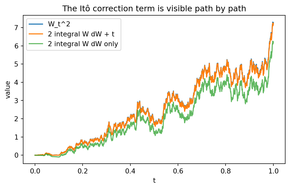
The next interactive experiment simulates one Brownian path. It compares the path $W_t^2$ with the Itô decomposition
$$
W_t^2 = 2\int_0^t W_s\,dW_s + t.
$$
The stochastic integral is approximated by left-endpoint sums.
::: {.interactive-card}
### Explore the identity $W_t^2=2\int_0^t W_s\,dW_s+t$
<div class="mf-controls">
<label for="ch12-n">number of time steps</label>
<input id="ch12-n" type="range" min="100" max="2000" step="100" value="800">
<label for="ch12-seed">path seed</label>
<input id="ch12-seed" type="range" min="1" max="20" step="1" value="7">
</div>
<div id="ch12-ito-correction-values" class="mf-output"></div>
<div id="ch12-ito-correction-plot" class="plotly-demo"></div>
<script>
window.mfPlotlyReady(function() {
const nSlider = document.getElementById('ch12-n');
const seedSlider = document.getElementById('ch12-seed');
const out = document.getElementById('ch12-ito-correction-values');
const plot = document.getElementById('ch12-ito-correction-plot');
function rngFactory(seed) {
let s = seed * 1234567 + 890123;
return function() {
s = (1664525 * s + 1013904223) >>> 0;
return s / 4294967296;
};
}
function normalPair(rand) {
const u1 = Math.max(rand(), 1e-12);
const u2 = rand();
const r = Math.sqrt(-2 * Math.log(u1));
return [r * Math.cos(2 * Math.PI * u2), r * Math.sin(2 * Math.PI * u2)];
}
function simulate(n, seed) {
const rand = rngFactory(seed);
const T = 1.0;
const dt = T / n;
const t = [0.0];
const W = [0.0];
let zCache = [];
for (let i = 0; i < n; i++) {
if (zCache.length === 0) zCache = normalPair(rand);
const z = zCache.pop();
t.push((i + 1) * dt);
W.push(W[W.length - 1] + Math.sqrt(dt) * z);
}
const leftIntegral = [0.0];
let acc = 0.0;
for (let i = 0; i < n; i++) {
acc += W[i] * (W[i + 1] - W[i]);
leftIntegral.push(acc);
}
const W2 = W.map(x => x * x);
const itoRecon = leftIntegral.map((v, i) => 2 * v + t[i]);
const ordinaryRecon = leftIntegral.map(v => 2 * v);
return {t, W, W2, itoRecon, ordinaryRecon, leftIntegral};
}
function update() {
const n = Number(nSlider.value);
const seed = Number(seedSlider.value);
const d = simulate(n, seed);
const finalErrorIto = Math.abs(d.W2[d.W2.length - 1] - d.itoRecon[d.itoRecon.length - 1]);
const finalErrorOrdinary = Math.abs(d.W2[d.W2.length - 1] - d.ordinaryRecon[d.ordinaryRecon.length - 1]);
out.innerHTML = 'steps = ' + n +
', final error with Itô correction = ' + finalErrorIto.toFixed(5) +
', final error without correction = ' + finalErrorOrdinary.toFixed(5) + '.';
Plotly.newPlot(plot, [
{x: d.t, y: d.W2, mode: 'lines', name: 'W_t^2'},
{x: d.t, y: d.itoRecon, mode: 'lines', name: '2 integral W dW + t'},
{x: d.t, y: d.ordinaryRecon, mode: 'lines', name: '2 integral W dW only'}
], {
title: 'Itô Correction for f(W)=W^2',
xaxis: {title: 't'},
yaxis: {title: 'value'},
margin: {l: 55, r: 20, t: 50, b: 50},
legend: {orientation: 'h'}
}, {responsive: true});
}
nSlider.addEventListener('input', update);
seedSlider.addEventListener('input', update);
update();
});
</script>
:::
## 12.7 Python Example: Verifying the Correction Term
```{python}
#| label: ch12-python-ito-correction
#| echo: true
import numpy as np
import matplotlib.pyplot as plt

rng = np.random.default_rng(7243)
T = 1.0
n = 2000
dt = T / n
t = np.linspace(0, T, n + 1)
dW = rng.normal(0.0, np.sqrt(dt), size=n)
W = np.concatenate([[0.0], np.cumsum(dW)])

ito_integral = np.concatenate([[0.0], np.cumsum(W[:-1] * dW)])
ito_reconstruction = 2 * ito_integral + t
ordinary_reconstruction = 2 * ito_integral

print("Final W_T^2:", W[-1] ** 2)
print("Final Itô reconstruction:", ito_reconstruction[-1])
print("Final ordinary-chain-rule reconstruction:", ordinary_reconstruction[-1])
print("Error with correction:", abs(W[-1] ** 2 - ito_reconstruction[-1]))
print("Error without correction:", abs(W[-1] ** 2 - ordinary_reconstruction[-1]))

plt.figure(figsize=(7, 4))
plt.plot(t, W**2, label="W_t^2")
plt.plot(t, ito_reconstruction, label="2 integral W dW + t")
plt.plot(t, ordinary_reconstruction, label="2 integral W dW only", alpha=0.75)
plt.xlabel("t")
plt.ylabel("value")
plt.title("The Itô correction term is visible path by path")
plt.legend()
plt.show()
```
The numerical approximation improves as the time grid becomes finer, but the ordinary-chain-rule reconstruction remains systematically wrong because it omits the accumulated quadratic variation.
## 12.8 Exponential Functions and Exponential Martingales
Let
$$
Y_t=e^{\theta W_t}.
$$
For $f(x)=e^{\theta x}$,
$$
f_x(x)=\theta e^{\theta x},
\qquad
f_{xx}(x)=\theta^2 e^{\theta x}.
$$
Itô's formula gives
$$
d(e^{\theta W_t})
=
\theta e^{\theta W_t}\,dW_t
+
\frac12\theta^2 e^{\theta W_t}\,dt.
$$
The process $e^{\theta W_t}$ has positive drift. To remove this drift, define
$$
M_t=\exp\left(\theta W_t-\frac12\theta^2t\right).
$$
Applying Itô's formula to $f(t,x)=\exp(\theta x-\frac12\theta^2t)$ yields
$$
dM_t=\theta M_t\,dW_t.
$$
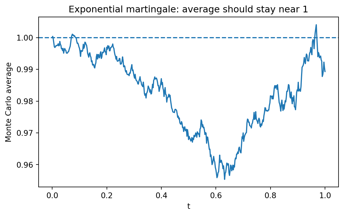
Therefore $M_t$ has zero drift and is a martingale.
::: {.example}
### Example 12.2: Moment generating function of Brownian motion
Since $M_t$ is a martingale and $M_0=1$,
$$
E[M_t]=1.
$$
Hence
$$
E[e^{\theta W_t}]=e^{\frac12\theta^2t}.
$$
This is the moment generating function of $N(0,t)$.
:::
```{python}
#| label: ch12-python-exponential-martingale
#| echo: true
import numpy as np
import matplotlib.pyplot as plt

rng = np.random.default_rng(5110)
T = 1.0
n = 500
m = 5000
theta = 1.25

dt = T / n
t = np.linspace(0, T, n + 1)
dW = rng.normal(0.0, np.sqrt(dt), size=(m, n))
W = np.concatenate([np.zeros((m, 1)), np.cumsum(dW, axis=1)], axis=1)

M = np.exp(theta * W - 0.5 * theta**2 * t)
mean_M = M.mean(axis=0)

print("Estimated E[M_T]:", mean_M[-1])
print("Theoretical E[M_T]:", 1.0)

plt.figure(figsize=(7, 4))
plt.plot(t, mean_M)
plt.axhline(1.0, linestyle="--")
plt.xlabel("t")
plt.ylabel("Monte Carlo average")
plt.title("Exponential martingale: average should stay near 1")
plt.show()
```
## 12.9 Applying Itô's Formula to Geometric Brownian Motion
The basic Black--Scholes stock model is
$$
dS_t=\mu S_t\,dt+\sigma S_t\,dW_t,
\qquad S_0>0.
$$
This is geometric Brownian motion. To solve it, apply Itô's formula to
$$
X_t=\log S_t.
$$
Let $f(s)=\log s$. Then
$$
f'(s)=\frac1s,
\qquad
f''(s)=-\frac1{s^2}.
$$
Since
$$
(dS_t)^2=\sigma^2S_t^2\,dt,
$$
Itô's formula gives
$$
d\log S_t
=
\frac1{S_t}dS_t-�rac12\frac1{S_t^2}(dS_t)^2.
$$
Substitute the SDE for $S_t$:
$$
d\log S_t
=
\left(\mu-�rac12\sigma^2\right)dt+
\sigma\,dW_t.
$$
Integrating from $0$ to $t$ gives
$$
\log S_t
=
\log S_0+
\left(\mu-�rac12\sigma^2\right)t+
\sigma W_t.
$$
Therefore
$$
S_t
=
S_0\exp\left(\left(\mu-�rac12\sigma^2\right)t+
\sigma W_t\right).
$$
::: {.callout-important}
## The volatility correction
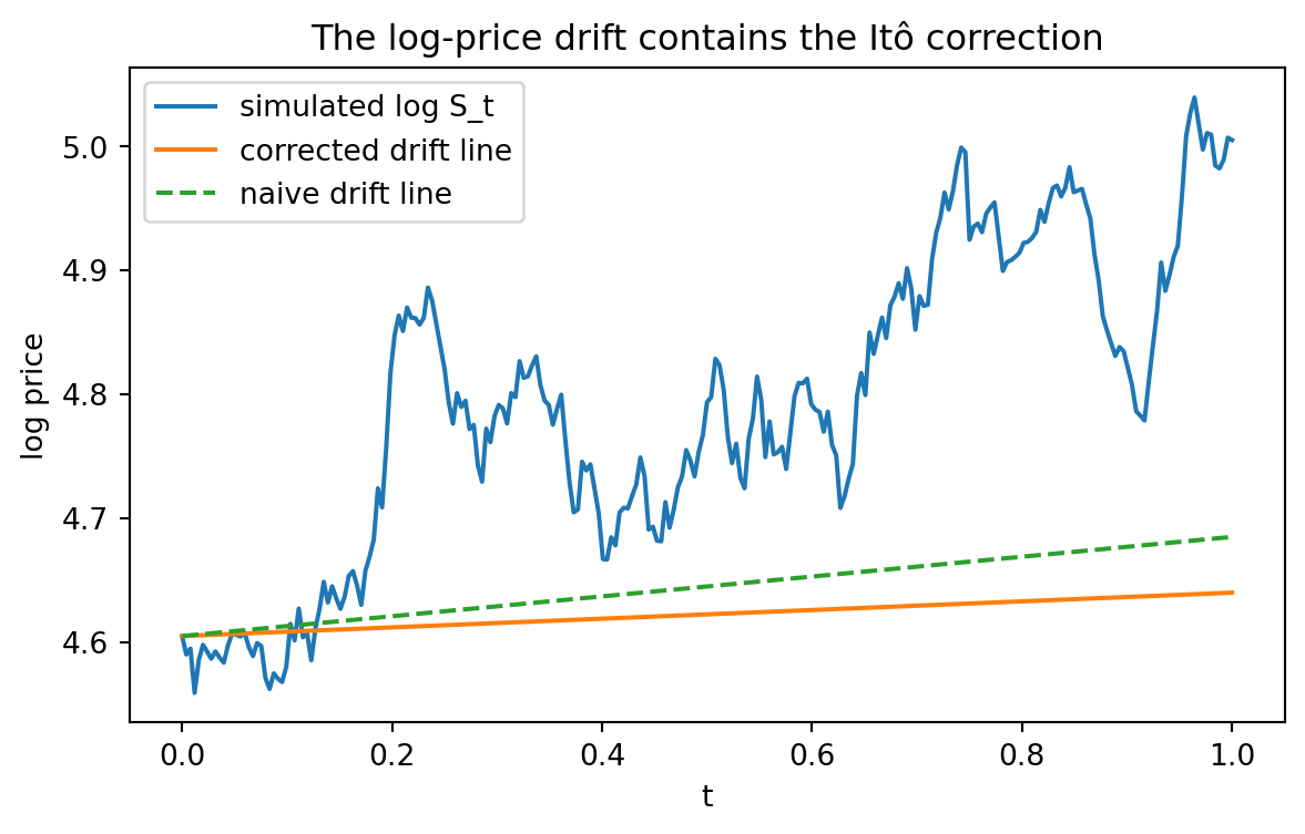
The drift of $\log S_t$ is not $\mu$. It is
$$
\mu-\frac12\sigma^2.
$$
This correction appears because the logarithm is concave and Brownian-driven prices have quadratic variation.
:::
## 12.10 Interactive Demo: Log Prices Under GBM
Move the sliders to see how the volatility correction changes the log-price drift.
::: {.interactive-card}
### Explore $d\log S_t=(\mu-\frac12\sigma^2)dt+\sigma dW_t$
<div class="mf-controls">
<label for="ch12-mu">drift $\mu$</label>
<input id="ch12-mu" type="range" min="-0.10" max="0.30" step="0.01" value="0.08">
<label for="ch12-sigma">volatility $\sigma$</label>
<input id="ch12-sigma" type="range" min="0.05" max="0.80" step="0.01" value="0.30">
<label for="ch12-gbm-seed">path seed</label>
<input id="ch12-gbm-seed" type="range" min="1" max="30" step="1" value="11">
</div>
<div id="ch12-gbm-values" class="mf-output"></div>
<div id="ch12-gbm-plot" class="plotly-demo"></div>
<script>
window.mfPlotlyReady(function() {
const muSlider = document.getElementById('ch12-mu');
const sigmaSlider = document.getElementById('ch12-sigma');
const seedSlider = document.getElementById('ch12-gbm-seed');
const out = document.getElementById('ch12-gbm-values');
const plot = document.getElementById('ch12-gbm-plot');
function rngFactory(seed) {
let s = seed * 9876543 + 12345;
return function() {
s = (1103515245 * s + 12345) >>> 0;
return s / 4294967296;
};
}
function normalPair(rand) {
const u1 = Math.max(rand(), 1e-12);
const u2 = rand();
const r = Math.sqrt(-2 * Math.log(u1));
return [r * Math.cos(2 * Math.PI * u2), r * Math.sin(2 * Math.PI * u2)];
}
function simulate(mu, sigma, seed) {
const S0 = 100;
const T = 1;
const n = 400;
const dt = T / n;
const rand = rngFactory(seed);
let zCache = [];
const t = [0.0];
const W = [0.0];
for (let i = 0; i < n; i++) {
if (zCache.length === 0) zCache = normalPair(rand);
const z = zCache.pop();
t.push((i + 1) * dt);
W.push(W[W.length - 1] + Math.sqrt(dt) * z);
}
const logS = t.map((x, i) => Math.log(S0) + (mu - 0.5 * sigma * sigma) * x + sigma * W[i]);
const S = logS.map(Math.exp);
const naiveLogMean = t.map(x => Math.log(S0) + mu * x);
const correctedLogMean = t.map(x => Math.log(S0) + (mu - 0.5 * sigma * sigma) * x);
return {t, S, logS, naiveLogMean, correctedLogMean};
}
function update() {
const mu = Number(muSlider.value);
const sigma = Number(sigmaSlider.value);
const seed = Number(seedSlider.value);
const d = simulate(mu, sigma, seed);
const logDrift = mu - 0.5 * sigma * sigma;
out.innerHTML = 'mu = ' + mu.toFixed(2) +
', sigma = ' + sigma.toFixed(2) +
', log-price drift = mu - sigma^2/2 = ' + logDrift.toFixed(4) + '.';
Plotly.newPlot(plot, [
{x: d.t, y: d.logS, mode: 'lines', name: 'simulated log S_t'},
{x: d.t, y: d.correctedLogMean, mode: 'lines', name: 'corrected log drift'},
{x: d.t, y: d.naiveLogMean, mode: 'lines', name: 'naive drift without correction'},
{x: d.t, y: d.S.map(s => Math.log(s)), mode: 'lines', name: 'log of simulated S_t', visible: 'legendonly'}
], {
title: 'Itô Correction in Geometric Brownian Motion',
xaxis: {title: 't'},
yaxis: {title: 'log price'},
margin: {l: 55, r: 20, t: 50, b: 50},
legend: {orientation: 'h'}
}, {responsive: true});
}
muSlider.addEventListener('input', update);
sigmaSlider.addEventListener('input', update);
seedSlider.addEventListener('input', update);
update();
});
</script>
:::
```{python}
#| label: ch12-python-gbm-log-transform
#| echo: true
import numpy as np
import matplotlib.pyplot as plt

rng = np.random.default_rng(2026)
S0 = 100.0
mu = 0.08
sigma = 0.30
T = 1.0
n = 252
dt = T / n
t = np.linspace(0, T, n + 1)

dW = rng.normal(0.0, np.sqrt(dt), size=n)
W = np.concatenate([[0.0], np.cumsum(dW)])
S_exact = S0 * np.exp((mu - 0.5 * sigma**2) * t + sigma * W)
logS = np.log(S_exact)

corrected_line = np.log(S0) + (mu - 0.5 * sigma**2) * t
naive_line = np.log(S0) + mu * t

print("log-price drift:", mu - 0.5 * sigma**2)
print("naive drift:", mu)
print("difference:", 0.5 * sigma**2)

plt.figure(figsize=(7, 4))
plt.plot(t, logS, label="simulated log S_t")
plt.plot(t, corrected_line, label="corrected drift line")
plt.plot(t, naive_line, label="naive drift line", linestyle="--")
plt.xlabel("t")
plt.ylabel("log price")
plt.title("The log-price drift contains the Itô correction")
plt.legend()
plt.show()
```
## 12.11 Powers of a Geometric Brownian Motion
Let
$$
dS_t=\mu S_t\,dt+\sigma S_t\,dW_t.
$$
For a power function
$$
f(s)=s^\alpha,
$$
we have
$$
f'(s)=\alpha s^{\alpha-1},
\qquad
f''(s)=\alpha(\alpha-1)s^{\alpha-2}.
$$
Itô's formula gives
$$
d(S_t^\alpha)
=
\alpha S_t^{\alpha-1}dS_t
+
\frac12\alpha(\alpha-1)S_t^{\alpha-2}(dS_t)^2.
$$
Because
$$
(dS_t)^2=\sigma^2S_t^2\,dt,
$$
we obtain
$$
d(S_t^\alpha)
=
\left(\alpha\mu+�rac12\alpha(\alpha-1)\sigma^2\right)S_t^\alpha\,dt
+
\alpha\sigma S_t^\alpha\,dW_t.
$$
This example shows how curvature changes drift. For $\alpha=1$, the correction vanishes. For $\alpha=0$, the process is constant. For $\alpha=2$, the correction is positive.
## 12.12 Product Rule and Integration by Parts
Let $X_t$ and $Y_t$ be Itô processes
$$
dX_t=\mu_t^X\,dt+\sigma_t^X\,dW_t,
$$
$$
dY_t=\mu_t^Y\,dt+\sigma_t^Y\,dW_t.
$$
Apply Itô's formula to $f(x,y)=xy$. Since
$$
f_x=y,
\qquad
f_y=x,
\qquad
f_{xy}=1,
$$
we get the stochastic product rule
$$
d(X_tY_t)=X_t\,dY_t+Y_t\,dX_t+dX_t\,dY_t.
$$
The cross term is
$$
dX_t\,dY_t=\sigma_t^X\sigma_t^Y\,dt.
$$
Thus
$$
d(X_tY_t)=X_t\,dY_t+Y_t\,dX_t+\sigma_t^X\sigma_t^Y\,dt.
$$
This is the stochastic integration-by-parts formula.
::: {.example}
### Example 12.3: Product of Brownian motion with itself
Take $X_t=Y_t=W_t$. Then
$$
d(W_t^2)=W_t\,dW_t+W_t\,dW_t+dW_t\,dW_t.
$$
Since $dW_t\,dW_t=dt$,
$$
d(W_t^2)=2W_t\,dW_t+dt.
$$
:::
```{python}
#| label: ch12-python-product-rule
#| echo: true
import numpy as np

rng = np.random.default_rng(1212)
T = 1.0
n = 10000
dt = T / n
rho = 0.65

dB1 = rng.normal(0.0, np.sqrt(dt), size=n)
dB2_ind = rng.normal(0.0, np.sqrt(dt), size=n)
dB2 = rho * dB1 + np.sqrt(1 - rho**2) * dB2_ind

B1 = np.concatenate([[0.0], np.cumsum(dB1)])
B2 = np.concatenate([[0.0], np.cumsum(dB2)])

# Approximate quadratic covariation.
quad_cov = np.sum(dB1 * dB2)
print("Estimated [B1,B2]_T:", quad_cov)
print("Theoretical value rho*T:", rho * T)

# Product rule check: B1_T B2_T = integral B1 dB2 + integral B2 dB1 + [B1,B2]_T
int_B1_dB2 = np.sum(B1[:-1] * dB2)
int_B2_dB1 = np.sum(B2[:-1] * dB1)
left_side = B1[-1] * B2[-1]
right_side = int_B1_dB2 + int_B2_dB1 + quad_cov
print("left side:", left_side)
print("right side:", right_side)
print("absolute error:", abs(left_side - right_side))
```
## 12.13 Multidimensional Itô Formula
Many financial models involve several sources of randomness. Let
$$
dX_t^i=\mu_i(t,X_t)\,dt+\sum_{k=1}^m \sigma_{ik}(t,X_t)\,dW_t^k,
\qquad i=1,\ldots,d,
$$
where $W_t=(W_t^1,\ldots,W_t^m)$ is an $m$-dimensional Brownian motion. Write $a=\sigma\sigma^\top$, so
$$
a_{ij}(t,x)=\sum_{k=1}^m \sigma_{ik}(t,x)\sigma_{jk}(t,x).
$$
::: {.theorem}
### Theorem 12.2: Multidimensional Itô formula
For a smooth function $f(t,x_1,\ldots,x_d)$,
$$
df(t,X_t)
=
\left(
f_t+
\sum_{i=1}^d \mu_i f_{x_i}
+\frac12\sum_{i=1}^d\sum_{j=1}^d a_{ij} f_{x_i x_j}
\right)dt
+
\sum_{k=1}^m\left(\sum_{i=1}^d f_{x_i}\sigma_{ik}\right)dW_t^k.
$$
:::
The second-derivative terms are weighted by instantaneous covariance, not just variance. This matters in multi-asset option pricing, portfolio diffusion models, stochastic volatility models, and interest-rate models.
If $dX_t$ and $dY_t$ are driven by Brownian motions with instantaneous correlation $\rho$, then
$$
dX_t\,dY_t=\sigma_X(t)\sigma_Y(t)\rho\,dt.
$$
## 12.14 The Generator View
For the Itô process
$$
dX_t=\mu(t,X_t)\,dt+\sigma(t,X_t)\,dW_t,
$$
the differential form of Itô's formula is
$$
df(t,X_t)=\left(f_t+Lf\right)(t,X_t)\,dt+\sigma(t,X_t)f_x(t,X_t)\,dW_t,
$$
where the differential operator $L$ is
$$
Lf(t,x)=\mu(t,x)f_x(t,x)+\frac12\sigma^2(t,x)f_{xx}(t,x).
$$
::: {.definition}
### Definition 12.2: Infinitesimal generator
The operator
$$
L f(x)=\mu(x)f'(x)+\frac12\sigma^2(x)f''(x)
$$
is called the infinitesimal generator of the diffusion
$$
dX_t=\mu(X_t)\,dt+\sigma(X_t)\,dW_t.
$$
:::
The generator is important because it connects stochastic processes with partial differential equations. In mathematical finance, this connection leads directly to pricing PDEs.
## 12.15 Preview: Itô's Formula and the Black--Scholes PDE
Let the stock price satisfy the risk-neutral model
$$
dS_t=rS_t\,dt+\sigma S_t\,dW_t^Q.
$$
Suppose a derivative price is represented by a smooth function
$$
V_t=v(t,S_t).
$$
Itô's formula gives
$$
dV_t
=
\left(v_t+rS_t v_s+\frac12\sigma^2S_t^2v_{ss}\right)dt
+
\sigma S_t v_s\,dW_t^Q.
$$
If the discounted derivative price is a martingale under the risk-neutral measure, then
$$
e^{-rt}V_t
$$
has zero drift. This leads to
$$
v_t+rsv_s+\frac12\sigma^2s^2v_{ss}-rv=0.
$$
This is the Black--Scholes PDE. Later chapters will derive it again using delta hedging and martingale pricing.
::: {.callout-note}
## Why this chapter matters for pricing
Itô's formula is the bridge from stochastic price dynamics to equations for derivative prices. Without Itô's formula, the Black--Scholes PDE and delta hedging cannot be derived cleanly.
:::
```{python}
#| label: ch12-python-black-scholes-pde-terms
#| echo: true
import numpy as np
from math import log, sqrt, exp, erf

# Standard normal CDF without scipy.
def N(x):
    return 0.5 * (1.0 + erf(x / sqrt(2.0)))

def call_price(t, s, K, T, r, sigma):
    tau = T - t
    if tau <= 0:
        return max(s - K, 0.0)
    d1 = (log(s / K) + (r + 0.5 * sigma**2) * tau) / (sigma * sqrt(tau))
    d2 = d1 - sigma * sqrt(tau)
    return s * N(d1) - K * exp(-r * tau) * N(d2)

# Finite differences to check the Black-Scholes PDE residual numerically.
K = 100.0
T = 1.0
r = 0.04
sigma = 0.25
t = 0.35
s = 105.0
h_t = 1e-4
h_s = 1e-2

v = call_price(t, s, K, T, r, sigma)
v_t = (call_price(t + h_t, s, K, T, r, sigma) - call_price(t - h_t, s, K, T, r, sigma)) / (2 * h_t)
v_s = (call_price(t, s + h_s, K, T, r, sigma) - call_price(t, s - h_s, K, T, r, sigma)) / (2 * h_s)
v_ss = (call_price(t, s + h_s, K, T, r, sigma) - 2 * v + call_price(t, s - h_s, K, T, r, sigma)) / (h_s**2)

residual = v_t + r * s * v_s + 0.5 * sigma**2 * s**2 * v_ss - r * v

print("call price:", v)
print("PDE residual:", residual)
```
The finite-difference residual should be close to zero. The calculation is not a proof of the formula, but it helps students see how Itô's formula produces the PDE terms.
## 12.16 Common Mistakes
::: {.warning}
### Mistake 1: Using the ordinary chain rule
For Brownian motion,
$$
d(W_t^2)\ne 2W_t\,dW_t.
$$
The correct formula is
$$
d(W_t^2)=2W_t\,dW_t+dt.
$$
:::
::: {.warning}
### Mistake 2: Forgetting the sign of the logarithm correction
If
$$
dS_t=\mu S_t\,dt+\sigma S_t\,dW_t,
$$
then
$$
d\log S_t=\left(\mu-\frac12\sigma^2\right)dt+\sigma\,dW_t.
$$
The correction is negative because $\log s$ is concave.
:::
::: {.warning}
### Mistake 3: Treating $dW_t$ like $dt$
The rule $dW_t$ has mean zero does not mean $(dW_t)^2$ is negligible. The squared increments accumulate to time.
:::
::: {.warning}
### Mistake 4: Ignoring covariance in multiple dimensions
If two Brownian shocks are correlated, the cross term contributes to drift:
$$
dX_t\,dY_t=\rho\sigma_X\sigma_Y\,dt.
$$
:::
## 12.17 AI-Assisted Learning Components
::: {.ai-box}
### AI prompt: Explain the Itô correction
Ask an AI tool:
> Explain why $d(W_t^2)$ is not equal to $2W_t\,dW_t$. Use both Taylor expansion and quadratic variation. Then give a financial interpretation involving a function of a stock price.
Check whether the answer explicitly mentions that $(dW_t)^2$ contributes $dt$.
:::
::: {.ai-box}
### AI prompt: Audit a stochastic-calculus derivation
Give an AI tool the following incorrect derivation:
> If $dS_t=\mu S_tdt+\sigma S_tdW_t$, then $d\log S_t=(1/S_t)dS_t=\mu dt+\sigma dW_t$.
Ask it to find the mistake, repair the derivation, and explain why the correction has sign $-\frac12\sigma^2$.
:::
::: {.ai-box}
### AI prompt: Code review for simulation
Ask an AI tool to inspect a Python simulation verifying
$$
\int_0^T W_t\,dW_t=\frac12(W_T^2-T).
$$
The code should use left-endpoint sums. Ask the AI to identify whether the code accidentally uses right endpoints or future information.
:::
## 12.18 Exercises
### Conceptual Exercises
1. Explain in words why Brownian motion forces a correction to the ordinary chain rule.
2. What does the rule $(dW_t)^2=dt$ mean mathematically?
3. Why is the Itô correction term related to curvature of $f$?
4. In the formula for $d\log S_t$, why does volatility reduce the log drift?
5. Why does the product rule for Itô processes contain an extra term?
### Computational Exercises
6. Let $X_t=W_t$. Use Itô's formula to compute $d(W_t^3)$.
7. Let $X_t=W_t$. Use Itô's formula to compute $d(e^{aW_t})$.
8. Let $dX_t=\mu\,dt+\sigma\,dW_t$. Compute $d(X_t^2)$.
9. Let $dS_t=\mu S_tdt+\sigma S_tdW_t$. Compute $d(S_t^2)$.
10. Let $dS_t=\mu S_tdt+\sigma S_tdW_t$. Compute $d(S_t^\alpha)$.
### Proof Exercises
11. Prove that $W_t^2-t$ is a martingale using Itô's formula.
12. Prove that $\exp(\theta W_t-\frac12\theta^2t)$ is a martingale using Itô's formula.
13. Derive the product rule from the two-dimensional Itô formula.
14. Derive the generator $L$ for the diffusion $dX_t=\mu(X_t)dt+\sigma(X_t)dW_t$.
15. Starting from the risk-neutral stock model, derive the Black--Scholes PDE drift condition.
### Python Exercises
16. Simulate Brownian motion and verify numerically that $W_T^2$ is closer to $2\sum W_{t_i}\Delta W_i+T$ than to $2\sum W_{t_i}\Delta W_i$.
17. Simulate the exponential martingale $M_t=\exp(\theta W_t-\frac12\theta^2t)$ and estimate $E[M_t]$ at several times.
18. Simulate geometric Brownian motion using both the exact formula and Euler--Maruyama. Compare the two paths as the time step decreases.
19. Simulate two correlated Brownian motions and estimate their quadratic covariation.
20. Write a function that takes symbolic derivatives of a function $f$ and returns the drift and diffusion terms from Itô's formula for $dX_t=\mu dt+\sigma dW_t$.
### AI-Assisted Exercises
21. Ask an AI tool to derive $d(S_t^\alpha)$ for a geometric Brownian motion. Verify each derivative and each differential rule manually.
22. Ask an AI tool to explain the difference between Itô and ordinary calculus in one paragraph for finance students. Improve the explanation by adding a formula.
23. Ask an AI tool to generate Python code verifying the identity for $W_t^2$. Check whether the code uses left endpoints.
24. Ask an AI tool to derive the Black--Scholes PDE from Itô's formula. Identify which assumption is mathematical and which is financial.
25. Ask an AI tool to give three common errors in applying Itô's formula. Add one example to each error.
## 12.19 Chapter Summary
Itô's formula is the stochastic chain rule for Brownian-driven processes. If
$$
dX_t=\mu_t\,dt+\sigma_t\,dW_t,
$$
then
$$
df(t,X_t)
=
\left(f_t+\mu_t f_x+\frac12\sigma_t^2 f_{xx}\right)dt
+
\sigma_t f_x\,dW_t.
$$
The new term
$$
\frac12\sigma_t^2 f_{xx}\,dt
$$
comes from quadratic variation. It changes the drift of nonlinear transformations and is responsible for key financial formulas such as the log form of geometric Brownian motion and the Black--Scholes PDE.
The central lesson is simple but powerful: in stochastic calculus, curvature and volatility combine to create drift.