---
title: "Chapter 16. Black--Scholes Formula"
---
::: {.chapter-objectives}
## Learning Goals
By the end of this chapter, students should be able to:
- state the Black--Scholes formulas for European calls and puts;
- derive the call formula from risk-neutral lognormal integration;
- explain the probabilistic meaning of $d_1$ and $d_2$;
- derive put-call parity and use it as a formula check;
- compute and interpret the main Greeks: delta, gamma, theta, vega, and rho;
- distinguish option price, intrinsic value, time value, and discounted strike;
- implement the formula carefully in Python;
- invert the formula numerically to obtain implied volatility;
- understand why implied volatility is a model-based quote rather than directly observed volatility;
- use AI tools to audit formulas, test code, and explain parameter sensitivities.
:::
::: {.hero-box}
The Black--Scholes formula is the closed-form solution of the Black--Scholes pricing problem for European call and put options. Under the risk-neutral measure $\mathbb Q$, the stock follows
$$
dS_t=rS_t\,dt+\sigma S_t\,dW_t^{\mathbb Q}.
$$
For a European call with strike $K$ and maturity $T$, the time-zero price is
$$
C_0=S_0N(d_1)-Ke^{-rT}N(d_2),
$$
where
$$
d_1=\frac{\log(S_0/K)+(r+\frac12\sigma^2)T}{\sigma\sqrt T},
\qquad
d_2=d_1-\sigma\sqrt T.
$$
The formula is not just a computational recipe. It is a compact expression of no-arbitrage, martingale pricing, lognormal distributions, and dynamic replication.
:::
## 16.1 From PDE to Formula
Chapter 15 derived the Black--Scholes partial differential equation
$$
V_t+\frac12\sigma^2S^2V_{SS}+rSV_S-rV=0.
$$
For a European derivative with payoff $h(S_T)$, the terminal condition is
$$
V(T,S)=h(S).
$$
The Black--Scholes formula gives an explicit solution for two especially important payoff functions:
$$
h_{\text{call}}(S_T)=(S_T-K)^+,
$$
and
$$
h_{\text{put}}(S_T)=(K-S_T)^+.
$$
Here $x^+=\max(x,0)$.
There are two standard ways to obtain the formula:
1. solve the Black--Scholes PDE by transforming it into the heat equation;
2. use risk-neutral valuation and integrate the lognormal distribution.
In this chapter we focus mainly on the second approach because it is cleaner for students who already understand probability and conditional expectation.
::: {.callout-note}
## Central pricing principle
Under the Black--Scholes assumptions, the time-zero price of a European payoff $h(S_T)$ is
$$
V_0=e^{-rT}\mathbb E^{\mathbb Q}[h(S_T)].
$$
For a call option, $h(S_T)=(S_T-K)^+$. Therefore
$$
C_0=e^{-rT}\mathbb E^{\mathbb Q}[(S_T-K)^+].
$$
:::
## 16.2 Risk-Neutral Stock Dynamics
Under the physical measure $\mathbb P$, the stock may have drift $\mu$:
$$
dS_t=\mu S_t\,dt+\sigma S_t\,dW_t^{\mathbb P}.
$$
Under the risk-neutral measure $\mathbb Q$, the drift becomes the risk-free rate $r$:
$$
dS_t=rS_t\,dt+\sigma S_t\,dW_t^{\mathbb Q}.
$$
Therefore the explicit solution is
$$
S_T=S_0\exp\left[\left(r-\frac12\sigma^2\right)T+\sigma\sqrt{T}Z\right],
\qquad Z\sim N(0,1) \text{ under } \mathbb Q.
$$
Taking logarithms gives
$$
\log S_T \sim N\left(\log S_0+\left(r-\frac12\sigma^2\right)T,\,\sigma^2T\right).
$$
This lognormal distribution is the source of the closed-form expression.
::: {.definition}
### Definition 16.1: European call and put
A **European call option** with strike $K$ and maturity $T$ pays
$$
(S_T-K)^+.
$$
A **European put option** with strike $K$ and maturity $T$ pays
$$
(K-S_T)^+.
$$
The word European means that the option can be exercised only at maturity. This matters because early exercise is an optimal stopping problem, not a simple terminal-expectation problem.
:::
## 16.3 Deriving the Call Formula
The risk-neutral price of a call is
$$
C_0=e^{-rT}\mathbb E^{\mathbb Q}[(S_T-K)^+].
$$
Since the payoff is positive exactly when $S_T>K$,
$$
(S_T-K)^+=S_T1_{\{S_T>K\}}-K1_{\{S_T>K\}}.
$$
Thus
$$
C_0=e^{-rT}\mathbb E^{\mathbb Q}\left[S_T1_{\{S_T>K\}}\right]
-Ke^{-rT}\mathbb Q(S_T>K).
$$
The second term is simpler. Since
$$
\log S_T=\log S_0+\left(r-\frac12\sigma^2\right)T+\sigma\sqrt{T}Z,
$$
the event $S_T>K$ is equivalent to
$$
Z>\frac{\log(K/S_0)-(r-\frac12\sigma^2)T}{\sigma\sqrt T}.
$$
Define
$$
d_2=\frac{\log(S_0/K)+(r-\frac12\sigma^2)T}{\sigma\sqrt T}.
$$
Then
$$
\mathbb Q(S_T>K)=N(d_2).
$$
The first term requires a tilted normal integral. Using the identity
$$
\mathbb E[e^{aZ}1_{\{Z>b\}}]=e^{a^2/2}N(a-b),
\qquad Z\sim N(0,1),
$$
with $a=\sigma\sqrt T$, one obtains
$$
e^{-rT}\mathbb E^{\mathbb Q}\left[S_T1_{\{S_T>K\}}\right]=S_0N(d_1),
$$
where
$$
d_1=d_2+\sigma\sqrt T
=\frac{\log(S_0/K)+(r+\frac12\sigma^2)T}{\sigma\sqrt T}.
$$
Therefore
$$
C_0=S_0N(d_1)-Ke^{-rT}N(d_2).
$$
::: {.theorem}
### Theorem 16.1: Black--Scholes European call formula
Assume the Black--Scholes model with constant $r$ and $\sigma>0$. The time-zero price of a European call option with strike $K$ and maturity $T$ is
$$
C_0=S_0N(d_1)-Ke^{-rT}N(d_2),
$$
where
$$
d_1=\frac{\log(S_0/K)+(r+\frac12\sigma^2)T}{\sigma\sqrt T},
\qquad
d_2=d_1-\sigma\sqrt T.
$$
:::
::: {.remark}
### Interpretation of $N(d_2)$ and $N(d_1)$
The quantity $N(d_2)$ is the risk-neutral probability that the call finishes in the money:
$$
N(d_2)=\mathbb Q(S_T>K).
$$
The quantity $N(d_1)$ is not exactly the same probability under $\mathbb Q$. It is a probability under a tilted measure that weights states by the stock price. Financially, $N(d_1)$ is also the call delta in the Black--Scholes model.
:::
## 16.4 Deriving the Put Formula
A European put has payoff
$$
(K-S_T)^+.
$$
The direct risk-neutral expectation calculation gives
$$
P_0=Ke^{-rT}N(-d_2)-S_0N(-d_1).
$$
This can also be obtained from put-call parity, which is often the simplest derivation.
::: {.theorem}
### Theorem 16.2: Black--Scholes European put formula
Under the same assumptions, the time-zero price of a European put option with strike $K$ and maturity $T$ is
$$
P_0=Ke^{-rT}N(-d_2)-S_0N(-d_1).
$$
:::
## 16.5 Put-Call Parity
For every $S_T$, the terminal payoffs satisfy
$$
(S_T-K)^+-(K-S_T)^+=S_T-K.
$$
Therefore a long call and short put have the same terminal payoff as holding one share of stock and borrowing $Ke^{-rT}$ today to repay $K$ at maturity. By no-arbitrage,
$$
C_0-P_0=S_0-Ke^{-rT}.
$$
::: {.theorem}
### Theorem 16.3: Put-call parity
For European options on a non-dividend-paying stock,
$$
C_0-P_0=S_0-Ke^{-rT}.
$$
Equivalently,
$$
P_0=C_0-S_0+Ke^{-rT}.
$$
:::
::: {.example}
### Example 16.1: Numerical Black--Scholes price
Let
$$
S_0=100,\qquad K=105,\qquad r=0.04,\qquad \sigma=0.25,\qquad T=1.
$$
Then
$$
d_1=\frac{\log(100/105)+(0.04+0.5(0.25)^2)}{0.25},
$$
and
$$
d_2=d_1-0.25.
$$
The call price is
$$
C_0=100N(d_1)-105e^{-0.04}N(d_2).
$$
The put price can be computed either from its own formula or from put-call parity.
:::
```{python}
#| label: ch16-black-scholes-basic-price
#| fig-cap: "Black--Scholes call and put price for a single parameter set."
import math


def norm_cdf(x):
    return 0.5 * (1.0 + math.erf(x / math.sqrt(2.0)))


def black_scholes_call_put(S, K, r, sigma, T):
    if S <= 0 or K <= 0 or sigma <= 0 or T <= 0:
        raise ValueError("S, K, sigma, and T must be positive.")
    d1 = (math.log(S / K) + (r + 0.5 * sigma**2) * T) / (sigma * math.sqrt(T))
    d2 = d1 - sigma * math.sqrt(T)
    call = S * norm_cdf(d1) - K * math.exp(-r * T) * norm_cdf(d2)
    put = K * math.exp(-r * T) * norm_cdf(-d2) - S * norm_cdf(-d1)
    return call, put, d1, d2

S, K, r, sigma, T = 100.0, 105.0, 0.04, 0.25, 1.0
call, put, d1, d2 = black_scholes_call_put(S, K, r, sigma, T)

print(f"d1 = {d1:.6f}")
print(f"d2 = {d2:.6f}")
print(f"call = {call:.6f}")
print(f"put  = {put:.6f}")
print(f"parity check C - P = {call - put:.6f}")
print(f"S - K exp(-rT)    = {S - K * math.exp(-r * T):.6f}")
```
## 16.6 Intrinsic Value and Time Value
The intrinsic value of a call is
$$
(S_0-K)^+.
$$
The intrinsic value of a put is
$$
(K-S_0)^+.
$$
The option price is usually larger than intrinsic value because the option holder benefits from favorable future movement while having limited downside. The difference is called time value:
$$
\text{time value}=\text{option price}-\text{intrinsic value}.
$$
Time value is strongly affected by volatility and maturity. Higher volatility increases both call and put prices, because convex payoffs benefit from dispersion.
::: {.remark}
### Convexity intuition
The call payoff $h(S)=(S-K)^+$ is convex. For a convex payoff, uncertainty can increase expected payoff. This is one reason why option values increase with volatility in the Black--Scholes model.
:::
## 16.7 Interactive: Call and Put Prices
The following interactive example shows how European call and put prices change with the stock price. The dashed curves show intrinsic values. Move the controls to see how maturity, volatility, strike, and interest rate affect time value.
::: {.interactive-card}
### Interactive 16.1: Black--Scholes price curves
<div class="mf-controls">
<label for="ch16-price-K">Strike K</label>
<input id="ch16-price-K" type="range" min="60" max="140" step="1" value="100">
<span id="ch16-price-K-value">100</span>
<label for="ch16-price-sigma">Volatility sigma</label>
<input id="ch16-price-sigma" type="range" min="0.05" max="0.80" step="0.01" value="0.25">
<span id="ch16-price-sigma-value">0.25</span>
<label for="ch16-price-T">Maturity T</label>
<input id="ch16-price-T" type="range" min="0.05" max="3.00" step="0.05" value="1.00">
<span id="ch16-price-T-value">1.00</span>
<label for="ch16-price-r">Risk-free rate r</label>
<input id="ch16-price-r" type="range" min="0.00" max="0.12" step="0.005" value="0.04">
<span id="ch16-price-r-value">0.04</span>
</div>
<div id="ch16-price-demo" class="plotly-demo"></div>
<div id="ch16-price-output" class="mf-output"></div>
:::
<script>
window.mfPlotlyReady(function() {
var div = document.getElementById("ch16-price-demo");
if (!div) return;
function erfApprox(x) {
var sign = x >= 0 ? 1 : -1;
x = Math.abs(x);
var a1 = 0.254829592;
var a2 = -0.284496736;
var a3 = 1.421413741;
var a4 = -1.453152027;
var a5 = 1.061405429;
var p = 0.3275911;
var t = 1 / (1 + p * x);
var y = 1 - (((((a5 * t + a4) * t) + a3) * t + a2) * t + a1) * t * Math.exp(-x * x);
return sign * y;
}
function N(x) { return 0.5 * (1 + erfApprox(x / Math.sqrt(2))); }
function price(S, K, r, sigma, T) {
var d1 = (Math.log(S / K) + (r + 0.5 * sigma * sigma) * T) / (sigma * Math.sqrt(T));
var d2 = d1 - sigma * Math.sqrt(T);
var call = S * N(d1) - K * Math.exp(-r * T) * N(d2);
var put = K * Math.exp(-r * T) * N(-d2) - S * N(-d1);
return {call: call, put: put, d1: d1, d2: d2};
}
var ids = ["K", "sigma", "T", "r"];
function getValue(name) {
return parseFloat(document.getElementById("ch16-price-" + name).value);
}
function updateLabels() {
ids.forEach(function(name) {
var v = getValue(name);
var digits = name === "K" ? 0 : 3;
document.getElementById("ch16-price-" + name + "-value").textContent = v.toFixed(digits);
});
}
function draw() {
updateLabels();
var K = getValue("K");
var sigma = getValue("sigma");
var T = getValue("T");
var r = getValue("r");
var Svals = [];
var calls = [];
var puts = [];
var callIntrinsic = [];
var putIntrinsic = [];
for (var i = 30; i <= 180; i += 1) {
var S = i;
var out = price(S, K, r, sigma, T);
Svals.push(S);
calls.push(out.call);
puts.push(out.put);
callIntrinsic.push(Math.max(S - K, 0));
putIntrinsic.push(Math.max(K - S, 0));
}
var traces = [
{x: Svals, y: calls, mode: "lines", name: "call price"},
{x: Svals, y: puts, mode: "lines", name: "put price"},
{x: Svals, y: callIntrinsic, mode: "lines", name: "call intrinsic", line: {dash: "dash"}},
{x: Svals, y: putIntrinsic, mode: "lines", name: "put intrinsic", line: {dash: "dash"}}
];
Plotly.newPlot(div, traces, {
title: "Black--Scholes prices as functions of stock price",
xaxis: {title: "stock price S"},
yaxis: {title: "option value"},
margin: {l: 55, r: 20, t: 50, b: 50}
}, {responsive: true});
var at = price(100, K, r, sigma, T);
var parityGap = at.call - at.put - (100 - K * Math.exp(-r * T));
document.getElementById("ch16-price-output").innerHTML =
"At S = 100: call = " + at.call.toFixed(4) +
", put = " + at.put.toFixed(4) +
", d1 = " + at.d1.toFixed(4) +
", d2 = " + at.d2.toFixed(4) +
". Put-call parity error = " + parityGap.toExponential(2) + ".";
}
ids.forEach(function(name) {
document.getElementById("ch16-price-" + name).addEventListener("input", draw);
});
draw();
});
</script>
## 16.8 Greeks: Local Sensitivities
The Greeks are derivatives of the option price with respect to model inputs. They are not new pricing formulas; they are local sensitivity measures.
For a European call,
$$
C=S_0N(d_1)-Ke^{-rT}N(d_2).
$$
The main Greeks are:
$$
\Delta_C=\frac{\partial C}{\partial S_0}=N(d_1),
$$
$$
\Gamma_C=\frac{\partial^2 C}{\partial S_0^2}
=\frac{\varphi(d_1)}{S_0\sigma\sqrt T},
$$
$$
\text{Vega}_C=\frac{\partial C}{\partial \sigma}
=S_0\varphi(d_1)\sqrt T,
$$
$$
\Theta_C=\frac{\partial C}{\partial T_{\text{calendar}}}
=-\frac{S_0\varphi(d_1)\sigma}{2\sqrt T}-rKe^{-rT}N(d_2),
$$
and
$$
\rho_C=\frac{\partial C}{\partial r}=KTe^{-rT}N(d_2).
$$
Here
$$
\varphi(x)=\frac{1}{\sqrt{2\pi}}e^{-x^2/2}
$$
is the standard normal density.
::: {.warning}
### Sign convention for theta
There are two common conventions. In this book, $T$ denotes time to maturity. Many trading platforms report theta as sensitivity to the passage of calendar time, so it is usually the negative of $\partial C/\partial T$ when $T$ is time to maturity.
:::
For a European put,
$$
\Delta_P=N(d_1)-1,
$$
$$
\Gamma_P=\Gamma_C,
$$
$$
\text{Vega}_P=\text{Vega}_C,
$$
$$
\Theta_P=-\frac{S_0\varphi(d_1)\sigma}{2\sqrt T}+rKe^{-rT}N(-d_2),
$$
and
$$
\rho_P=-KTe^{-rT}N(-d_2).
$$
::: {.remark}
### Why calls and puts have the same gamma and vega
Put-call parity gives
$$
C-P=S_0-Ke^{-rT}.
$$
The right-hand side is linear in $S_0$ and independent of $\sigma$. Differentiating twice with respect to $S_0$ gives
$$
\Gamma_C-\Gamma_P=0.
$$
Differentiating with respect to $\sigma$ gives
$$
\text{Vega}_C-\text{Vega}_P=0.
$$
:::
```{python}
#| label: ch16-greeks-functions
#| fig-cap: "Black--Scholes price and Greeks implemented from scratch."
import math
import numpy as np
import pandas as pd


def n_pdf(x):
    return math.exp(-0.5 * x * x) / math.sqrt(2.0 * math.pi)


def N(x):
    return 0.5 * (1.0 + math.erf(x / math.sqrt(2.0)))


def bs_price_greeks(S, K, r, sigma, T, option="call"):
    d1 = (math.log(S / K) + (r + 0.5 * sigma**2) * T) / (sigma * math.sqrt(T))
    d2 = d1 - sigma * math.sqrt(T)
    discK = K * math.exp(-r * T)
    if option == "call":
        price = S * N(d1) - discK * N(d2)
        delta = N(d1)
        theta = -S * n_pdf(d1) * sigma / (2 * math.sqrt(T)) - r * discK * N(d2)
        rho = K * T * math.exp(-r * T) * N(d2)
    elif option == "put":
        price = discK * N(-d2) - S * N(-d1)
        delta = N(d1) - 1
        theta = -S * n_pdf(d1) * sigma / (2 * math.sqrt(T)) + r * discK * N(-d2)
        rho = -K * T * math.exp(-r * T) * N(-d2)
    else:
        raise ValueError("option must be 'call' or 'put'")
    gamma = n_pdf(d1) / (S * sigma * math.sqrt(T))
    vega = S * n_pdf(d1) * math.sqrt(T)
    return {
        "price": price,
        "delta": delta,
        "gamma": gamma,
        "vega": vega,
        "theta": theta,
        "rho": rho,
        "d1": d1,
        "d2": d2,
    }

rows = []
for option in ["call", "put"]:
    out = bs_price_greeks(100, 100, 0.04, 0.25, 1.0, option=option)
    rows.append({"option": option, **out})

pd.DataFrame(rows).round(6)
```
## 16.9 Interactive: Greeks Across Stock Price
Gamma and vega are largest near the strike when maturity is not too long. Delta changes most rapidly near the strike, and that rapid change is exactly what gamma measures.
::: {.interactive-card}
### Interactive 16.2: Greeks as functions of $S$
<div class="mf-controls">
<label for="ch16-greek-K">Strike K</label>
<input id="ch16-greek-K" type="range" min="60" max="140" step="1" value="100">
<span id="ch16-greek-K-value">100</span>
<label for="ch16-greek-sigma">Volatility sigma</label>
<input id="ch16-greek-sigma" type="range" min="0.05" max="0.80" step="0.01" value="0.25">
<span id="ch16-greek-sigma-value">0.25</span>
<label for="ch16-greek-T">Maturity T</label>
<input id="ch16-greek-T" type="range" min="0.05" max="3.00" step="0.05" value="1.00">
<span id="ch16-greek-T-value">1.00</span>
<label for="ch16-greek-r">Risk-free rate r</label>
<input id="ch16-greek-r" type="range" min="0.00" max="0.12" step="0.005" value="0.04">
<span id="ch16-greek-r-value">0.04</span>
</div>
<div id="ch16-greek-demo" class="plotly-demo"></div>
<div id="ch16-greek-output" class="mf-output"></div>
:::
<script>
window.mfPlotlyReady(function() {
var div = document.getElementById("ch16-greek-demo");
if (!div) return;
function erfApprox(x) {
var sign = x >= 0 ? 1 : -1;
x = Math.abs(x);
var a1 = 0.254829592;
var a2 = -0.284496736;
var a3 = 1.421413741;
var a4 = -1.453152027;
var a5 = 1.061405429;
var p = 0.3275911;
var t = 1 / (1 + p * x);
var y = 1 - (((((a5 * t + a4) * t) + a3) * t + a2) * t + a1) * t * Math.exp(-x * x);
return sign * y;
}
function N(x) { return 0.5 * (1 + erfApprox(x / Math.sqrt(2))); }
function phi(x) { return Math.exp(-0.5 * x * x) / Math.sqrt(2 * Math.PI); }
function greeks(S, K, r, sigma, T) {
var d1 = (Math.log(S / K) + (r + 0.5 * sigma * sigma) * T) / (sigma * Math.sqrt(T));
var d2 = d1 - sigma * Math.sqrt(T);
return {
delta: N(d1),
gamma: phi(d1) / (S * sigma * Math.sqrt(T)),
vega: S * phi(d1) * Math.sqrt(T),
d1: d1,
d2: d2
};
}
var ids = ["K", "sigma", "T", "r"];
function getValue(name) {
return parseFloat(document.getElementById("ch16-greek-" + name).value);
}
function updateLabels() {
ids.forEach(function(name) {
var v = getValue(name);
var digits = name === "K" ? 0 : 3;
document.getElementById("ch16-greek-" + name + "-value").textContent = v.toFixed(digits);
});
}
function draw() {
updateLabels();
var K = getValue("K");
var sigma = getValue("sigma");
var T = getValue("T");
var r = getValue("r");
var Svals = [];
var deltas = [];
var gammasScaled = [];
var vegasScaled = [];
for (var i = 30; i <= 180; i += 1) {
var S = i;
var g = greeks(S, K, r, sigma, T);
Svals.push(S);
deltas.push(g.delta);
gammasScaled.push(20 * g.gamma);
vegasScaled.push(g.vega / 100);
}
Plotly.newPlot(div, [
{x: Svals, y: deltas, mode: "lines", name: "call delta"},
{x: Svals, y: gammasScaled, mode: "lines", name: "20 x gamma"},
{x: Svals, y: vegasScaled, mode: "lines", name: "vega / 100"}
], {
title: "Selected Black--Scholes Greeks across stock price",
xaxis: {title: "stock price S"},
yaxis: {title: "scaled sensitivity"},
margin: {l: 55, r: 20, t: 50, b: 50}
}, {responsive: true});
var at = greeks(100, K, r, sigma, T);
document.getElementById("ch16-greek-output").innerHTML =
"At S = 100: call delta = " + at.delta.toFixed(4) +
", gamma = " + at.gamma.toFixed(5) +
", vega = " + at.vega.toFixed(4) + ".";
}
ids.forEach(function(name) {
document.getElementById("ch16-greek-" + name).addEventListener("input", draw);
});
draw();
});
</script>
## 16.10 Finite-Difference Checks for Greeks
The formulas for Greeks should be checked numerically. For example, delta can be approximated by a central difference:
$$
\Delta \approx \frac{C(S_0+h)-C(S_0-h)}{2h}.
$$
Gamma can be approximated by
$$
\Gamma \approx \frac{C(S_0+h)-2C(S_0)+C(S_0-h)}{h^2}.
$$
These checks are useful because sign errors in Greeks are common.
```{python}
#| label: ch16-finite-difference-greeks
#| fig-cap: "Finite-difference checks for delta and gamma."
S, K, r, sigma, T = 100.0, 100.0, 0.04, 0.25, 1.0
h = 0.01

base = bs_price_greeks(S, K, r, sigma, T, option="call")
C_plus = bs_price_greeks(S + h, K, r, sigma, T, option="call")["price"]
C_0 = base["price"]
C_minus = bs_price_greeks(S - h, K, r, sigma, T, option="call")["price"]

fd_delta = (C_plus - C_minus) / (2 * h)
fd_gamma = (C_plus - 2 * C_0 + C_minus) / (h**2)

print(f"analytic delta = {base['delta']:.8f}")
print(f"FD delta       = {fd_delta:.8f}")
print(f"analytic gamma = {base['gamma']:.8f}")
print(f"FD gamma       = {fd_gamma:.8f}")
```
## 16.11 Monte Carlo Check of the Formula
The call price can be estimated by simulating risk-neutral terminal stock prices:
$$
S_T=S_0\exp\left[\left(r-\frac12\sigma^2\right)T+\sigma\sqrt T Z\right].
$$
Then
$$
C_0\approx e^{-rT}\frac1M\sum_{m=1}^M(S_T^{(m)}-K)^+.
$$
This is not the most efficient way to price a plain European call, because the closed-form formula is available. However, Monte Carlo is important because it extends to many path-dependent and high-dimensional problems where no closed form is available.
```{python}
#| label: ch16-monte-carlo-check
#| fig-cap: "Monte Carlo check of the Black--Scholes call formula."
import numpy as np

rng = np.random.default_rng(7243)
S, K, r, sigma, T = 100.0, 100.0, 0.04, 0.25, 1.0
M = 200_000
Z = rng.standard_normal(M)
ST = S * np.exp((r - 0.5 * sigma**2) * T + sigma * np.sqrt(T) * Z)
payoff = np.maximum(ST - K, 0.0)
mc_price = np.exp(-r * T) * payoff.mean()
mc_se = np.exp(-r * T) * payoff.std(ddof=1) / np.sqrt(M)
formula_price = bs_price_greeks(S, K, r, sigma, T, option="call")["price"]

print(f"Black--Scholes formula = {formula_price:.6f}")
print(f"Monte Carlo estimate   = {mc_price:.6f}")
print(f"Monte Carlo s.e.       = {mc_se:.6f}")
print(f"z-score of error       = {(mc_price - formula_price) / mc_se:.3f}")
```
## 16.12 Implied Volatility
The Black--Scholes formula gives the option price when $\sigma$ is known. In the market, option prices are observed and volatility is often inferred from those prices.
::: {.definition}
### Definition 16.2: Implied volatility
Given a market call price $C^{\text{mkt}}$, the **Black--Scholes implied volatility** is a value $\sigma_{\text{imp}}>0$ such that
$$
C^{\text{mkt}}=C^{\text{BS}}(S_0,K,r,T,\sigma_{\text{imp}}).
$$
For a put, it is defined similarly using the put formula.
:::
Implied volatility is a model-based way of quoting option prices. It is not the same as historical volatility and is not directly observed. It is the volatility input that makes the Black--Scholes model reproduce an observed option price.
For a non-dividend-paying European call, the Black--Scholes call price is increasing in $\sigma$ because vega is positive:
$$
\frac{\partial C}{\partial \sigma}=S_0\varphi(d_1)\sqrt T>0.
$$
Therefore, under valid no-arbitrage bounds, implied volatility is unique.
The no-arbitrage bounds for a European call are
$$
(S_0-Ke^{-rT})^+\le C_0\le S_0.
$$
For a put they are
$$
(Ke^{-rT}-S_0)^+\le P_0\le Ke^{-rT}.
$$
```{python}
#| label: ch16-implied-volatility
#| fig-cap: "Bisection method for Black--Scholes implied volatility."
def implied_vol_call(C_market, S, K, r, T, tol=1e-10, max_iter=200):
    lower_bound = max(S - K * math.exp(-r * T), 0.0)
    upper_bound = S
    if not (lower_bound <= C_market <= upper_bound):
        raise ValueError("Market price violates no-arbitrage call bounds.")

    lo, hi = 1e-8, 5.0
    for _ in range(max_iter):
        mid = 0.5 * (lo + hi)
        C_mid = bs_price_greeks(S, K, r, mid, T, option="call")["price"]
        if abs(C_mid - C_market) < tol:
            return mid
        if C_mid < C_market:
            lo = mid
        else:
            hi = mid
    return 0.5 * (lo + hi)

S, K, r, T = 100.0, 100.0, 0.04, 1.0
true_sigma = 0.32
market_price = bs_price_greeks(S, K, r, true_sigma, T, option="call")["price"]
recovered_sigma = implied_vol_call(market_price, S, K, r, T)

print(f"market price generated from sigma = {true_sigma:.4f}")
print(f"market call price                 = {market_price:.6f}")
print(f"recovered implied volatility       = {recovered_sigma:.6f}")
```
## 16.13 Volatility Smile and Model Critique
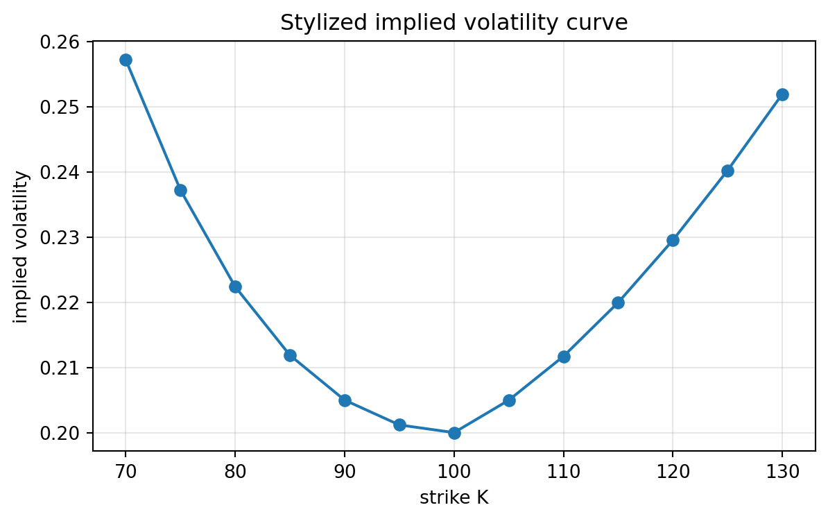
If the Black--Scholes model were exactly correct with constant volatility, all options on the same underlying and maturity would have the same implied volatility. In real markets, implied volatility often depends on strike and maturity. The graph of implied volatility against strike is called a volatility smile or skew.
A stylized smile can be created by assigning different prices to different strikes and then inverting the Black--Scholes formula. This does not prove that the market follows a different model, but it shows that the constant-volatility Black--Scholes model cannot fit all option prices with one value of $\sigma$.
```{python}
#| label: ch16-volatility-smile-demo
#| fig-cap: "A stylized implied-volatility smile."
import matplotlib.pyplot as plt

S, r, T = 100.0, 0.03, 0.75
strikes = np.arange(70.0, 131.0, 5.0)
# A stylized market volatility curve used only for demonstration.
market_sigmas = 0.20 + 0.45 * (np.log(strikes / S))**2 + 0.08 * np.maximum(np.log(strikes / S), 0)
market_prices = [bs_price_greeks(S, K, r, sig, T, option="call")["price"]
                 for K, sig in zip(strikes, market_sigmas)]
implied = [implied_vol_call(C, S, K, r, T) for C, K in zip(market_prices, strikes)]

plt.figure(figsize=(7, 4))
plt.plot(strikes, implied, marker="o")
plt.xlabel("strike K")
plt.ylabel("implied volatility")
plt.title("Stylized implied volatility curve")
plt.grid(True, alpha=0.3)
plt.show()
```
::: {.ai-box}
### AI-assisted model critique
Ask an AI assistant:
> In the Black--Scholes model, volatility is constant. In market data, implied volatility often varies by strike and maturity. Explain why this creates a model-risk issue. Do not recommend a trading strategy. Focus on the mathematical inconsistency between a one-parameter volatility model and a surface of quoted implied volatilities.
Then check whether the response correctly distinguishes:
1. historical volatility;
2. model volatility;
3. implied volatility;
4. local or stochastic volatility as possible model extensions.
:::
## 16.14 Dividends and Foreign Exchange Variant
If the stock pays a continuous dividend yield $q$, the risk-neutral stock dynamics become
$$
dS_t=(r-q)S_t\,dt+\sigma S_t\,dW_t^{\mathbb Q}.
$$
The European call and put formulas become
$$
C_0=S_0e^{-qT}N(d_1)-Ke^{-rT}N(d_2),
$$
and
$$
P_0=Ke^{-rT}N(-d_2)-S_0e^{-qT}N(-d_1),
$$
where
$$
d_1=\frac{\log(S_0/K)+(r-q+\frac12\sigma^2)T}{\sigma\sqrt T},
\qquad d_2=d_1-\sigma\sqrt T.
$$
Put-call parity becomes
$$
C_0-P_0=S_0e^{-qT}-Ke^{-rT}.
$$
This same structure is used for foreign exchange options by interpreting $q$ as the foreign risk-free rate.
## 16.15 Numerical Stability and Edge Cases
A good implementation should handle limiting cases carefully.
As $T\to 0$, the option value approaches intrinsic value:
$$
C_0\to (S_0-K)^+,
\qquad
P_0\to (K-S_0)^+.
$$
As $\sigma\to 0$, the risk-neutral terminal stock becomes deterministic:
$$
S_T=S_0e^{rT}.
$$
Hence
$$
C_0\to e^{-rT}(S_0e^{rT}-K)^+=(S_0-Ke^{-rT})^+.
$$
A robust implementation should avoid division by zero when $T$ or $\sigma$ is extremely small.
```{python}
#| label: ch16-robust-bs-function
#| fig-cap: "A robust Black--Scholes function with limiting cases."
def robust_bs_price(S, K, r, sigma, T, option="call"):
    if S <= 0 or K <= 0:
        raise ValueError("S and K must be positive.")
    if T <= 1e-12:
        return max(S - K, 0.0) if option == "call" else max(K - S, 0.0)
    if sigma <= 1e-12:
        forward = S * math.exp(r * T)
        payoff = max(forward - K, 0.0) if option == "call" else max(K - forward, 0.0)
        return math.exp(-r * T) * payoff
    return bs_price_greeks(S, K, r, sigma, T, option=option)["price"]

for T_small, sigma_small in [(1e-14, 0.25), (1.0, 1e-14), (1.0, 0.25)]:
    print(T_small, sigma_small, robust_bs_price(100, 100, 0.04, sigma_small, T_small, "call"))
```
## 16.16 Formula Verification by PDE Residual
The call formula should solve the Black--Scholes PDE:
$$
C_t+\frac12\sigma^2S^2C_{SS}+rSC_S-rC=0.
$$
When using time to maturity $\tau=T-t$, write the price as $C(S,\tau)$. Since $C_t=-C_\tau$, the PDE becomes
$$
-C_\tau+\frac12\sigma^2S^2C_{SS}+rSC_S-rC=0.
$$
This is a good way to check signs. In particular, students often accidentally use $+C_\tau$ in the PDE when the variable is time to maturity.
```{python}
#| label: ch16-pde-residual-check
#| fig-cap: "Numerical PDE residual check using finite differences."
def call_price_tau(S, K, r, sigma, tau):
    return robust_bs_price(S, K, r, sigma, tau, option="call")

S, K, r, sigma, tau = 110.0, 100.0, 0.04, 0.25, 0.8
hS = 0.05
ht = 1e-4

C = call_price_tau(S, K, r, sigma, tau)
C_plus_S = call_price_tau(S + hS, K, r, sigma, tau)
C_minus_S = call_price_tau(S - hS, K, r, sigma, tau)
C_plus_tau = call_price_tau(S, K, r, sigma, tau + ht)
C_minus_tau = call_price_tau(S, K, r, sigma, tau - ht)

C_S = (C_plus_S - C_minus_S) / (2 * hS)
C_SS = (C_plus_S - 2 * C + C_minus_S) / (hS**2)
C_tau = (C_plus_tau - C_minus_tau) / (2 * ht)

residual = -C_tau + 0.5 * sigma**2 * S**2 * C_SS + r * S * C_S - r * C
print(f"PDE residual = {residual:.6e}")
```
## 16.17 Common Mistakes
1. **Using $\mu$ in the Black--Scholes formula.** The formula uses $r$, not the physical drift $\mu$.
2. **Forgetting the discount factor.** The strike term is $Ke^{-rT}$, not $K$.
3. **Confusing $d_1$ and $d_2$.** The stock term uses $N(d_1)$; the strike term uses $N(d_2)$.
4. **Treating $N(d_1)$ as the risk-neutral exercise probability.** The risk-neutral exercise probability is $N(d_2)$.
5. **Confusing vega units.** The mathematical derivative is per unit volatility. Market convention often reports vega per one volatility point, which is one percent.
6. **Ignoring no-arbitrage bounds before computing implied volatility.** Invalid prices may not have a valid implied volatility.
7. **Using time-to-maturity signs incorrectly in theta or PDE checks.**
::: {.ai-box}
### AI-assisted formula audit
Ask an AI assistant to check the following intentionally suspicious claim:
> The Black--Scholes call price is $C=S_0N(d_2)-Ke^{-rT}N(d_1)$, and $N(d_1)$ is the risk-neutral probability that the option expires in the money.
Your task is to identify every error. A correct critique should say:
- the stock term uses $N(d_1)$;
- the strike term uses $N(d_2)$;
- $N(d_2)$ is the risk-neutral in-the-money probability;
- $N(d_1)$ has a different tilted-measure interpretation and equals call delta.
:::
::: {.ai-box}
### AI-assisted code review
Paste your Black--Scholes implementation into an AI assistant and ask it to design tests. The tests should include:
1. put-call parity;
2. monotonicity in $S$;
3. monotonicity in $\sigma$;
4. limiting behavior as $T\to 0$;
5. finite-difference checks of delta and gamma;
6. no-arbitrage bounds for calls and puts.
Do not ask the AI to simply rewrite the code. Ask it to find mathematical tests that would reveal implementation errors.
:::
## 16.18 Exercises
### Conceptual exercises
1. Explain why the Black--Scholes formula uses $r$ instead of the physical drift $\mu$.
2. Explain why call and put prices increase with volatility under the Black--Scholes model.
3. Explain why $N(d_2)$ is a probability but $N(d_1)$ should not be interpreted as the same probability.
4. What happens to the call price when $T\to 0$? What happens when $\sigma\to 0$?
5. Explain why implied volatility is not the same object as historical realized volatility.
### Mathematical exercises
6. Starting from
$$
C_0=e^{-rT}\mathbb E^{\mathbb Q}[(S_T-K)^+],
$$
derive the Black--Scholes call formula by splitting the payoff into
$$
S_T1_{\{S_T>K\}}-K1_{\{S_T>K\}}.
$$
7. Prove put-call parity by comparing terminal payoffs.
8. Differentiate the call formula with respect to $S_0$ and show that $\Delta_C=N(d_1)$.
9. Use put-call parity to derive the put delta from the call delta.
10. Show that call and put gamma are equal.
11. Show that call and put vega are equal.
12. Derive the no-arbitrage bounds
$$
(S_0-Ke^{-rT})^+\le C_0\le S_0.
$$
### Computational exercises
13. Implement the Black--Scholes call and put formulas without using `scipy.stats`.
14. Verify put-call parity numerically for at least five different parameter choices.
15. Plot call price as a function of $S_0$ for several values of $\sigma$.
16. Plot delta, gamma, and vega as functions of $S_0$.
17. Write a bisection solver for implied volatility and test it on synthetic option prices.
18. Simulate the risk-neutral terminal stock price and compare Monte Carlo estimates with the formula.
19. Use finite differences to check delta, gamma, and vega.
20. Create a stylized implied-volatility smile and explain why one constant volatility cannot fit it.
### AI-assisted exercises
21. Ask an AI assistant to explain the difference between $d_1$ and $d_2$. Then rewrite the explanation in your own words and correct any overstatements.
22. Ask an AI assistant to generate unit tests for a Black--Scholes function. Keep only the tests that have a clear mathematical reason.
23. Ask an AI assistant to critique the assumptions of Black--Scholes. Separate mathematical assumptions from market microstructure issues.
24. Ask an AI assistant to explain why vega is positive. Check whether the explanation uses convexity, differentiation, or both.
## 16.19 Chapter Summary
The Black--Scholes formula is the closed-form expression for European call and put prices in the constant-volatility complete-market model. It can be derived from the Black--Scholes PDE or from risk-neutral expectation under lognormal stock dynamics.
The call formula is
$$
C_0=S_0N(d_1)-Ke^{-rT}N(d_2),
$$
and the put formula is
$$
P_0=Ke^{-rT}N(-d_2)-S_0N(-d_1).
$$
The formula is mathematically elegant because it compresses several ideas into one expression: no-arbitrage, discounting, lognormal distributions, martingale pricing, and dynamic hedging. The Greeks measure local sensitivities of the formula, while implied volatility reverses the formula to express market prices in volatility units.
The next chapter studies change of measure and Girsanov's theorem, which explains more deeply why the physical Brownian motion under $\mathbb P$ can be transformed into a risk-neutral Brownian motion under $\mathbb Q$.