---
title: "Chapter 13. Stochastic Differential Equations"
---
::: {.chapter-objectives}
## Learning Goals
By the end of this chapter, students should be able to:
- read a stochastic differential equation as an integral equation;
- distinguish drift, diffusion coefficient, volatility, and Brownian noise;
- explain why adaptedness is essential in a financial model;
- state practical existence and uniqueness conditions for one-dimensional SDEs;
- solve the basic linear SDEs used in finance, including arithmetic Brownian motion, geometric Brownian motion, and Ornstein--Uhlenbeck dynamics;
- use Itô's formula to check proposed solutions of SDEs;
- simulate SDEs with the Euler--Maruyama method;
- distinguish exact simulation, approximate simulation, strong error, and weak error;
- interpret SDEs under physical and risk-neutral probability measures;
- use Python and AI tools to audit stochastic simulations and modeling assumptions.
:::
::: {.hero-box}
A stochastic differential equation, or SDE, has the informal form
$$
dX_t = b(t,X_t)\,dt + \sigma(t,X_t)\,dW_t.
$$
The rigorous meaning is the integral equation
$$
X_t = X_0 + \int_0^t b(s,X_s)\,ds + \int_0^t \sigma(s,X_s)\,dW_s.
$$
The first integral is ordinary time accumulation. The second integral is an Itô integral. Thus an SDE is not an ordinary differential equation with a rough input added at the end. It is a rule for constructing an adapted stochastic process whose local change contains both predictable drift and unpredictable Brownian shock.
:::
## 13.1 Why SDEs Enter Mathematical Finance
Financial prices move through time under uncertainty. A deterministic model such as
$$
\frac{dS_t}{dt}=\mu S_t
$$
says that the instantaneous growth rate is known. Its solution is
$$
S_t=S_0e^{\mu t}.
$$
This is useful for a bank account or a deterministic discount curve, but it cannot describe random market fluctuations. A natural idea is to add noise. In continuous time, Brownian motion is the basic model for accumulated small shocks. This leads to models such as
$$
dS_t=\mu S_t\,dt+\sigma S_t\,dW_t.
$$
Here $\mu$ is a drift parameter and $\sigma$ is a volatility parameter. The term $\mu S_t\,dt$ describes the local predictable component. The term $\sigma S_t\,dW_t$ describes the random component.
::: {.callout-note}
## Financial meaning
In asset pricing, an SDE is not only a path simulator. It specifies how information arrives and how risk enters the model. The drift determines expected growth under a chosen probability measure. The diffusion coefficient determines local risk exposure and is central to hedging.
:::
The central mathematical point is that Brownian paths are not differentiable. Therefore an expression such as $dW_t/dt$ is not an ordinary function. We do not define an SDE by differentiating Brownian motion. We define it through integrals.
## 13.2 Probability Space and Information
We work on a filtered probability space
$$
(\Omega,\mathcal F,(\mathcal F_t)_{t\ge 0},\mathbb P),
$$
where $W_t$ is a Brownian motion adapted to the filtration $(\mathcal F_t)$. The filtration represents available information. A process $X_t$ is adapted if $X_t$ is known at time $t$.
In finance, adaptedness prevents a trading strategy from using future information. If $X_t$ is a price process, then the model should specify how $X_t$ evolves using information available up to time $t$.
::: {.definition}
### Definition 13.1: SDE in integral form
Let $W_t$ be a Brownian motion. A process $X_t$ solves the SDE
$$
dX_t=b(t,X_t)\,dt+\sigma(t,X_t)\,dW_t, \qquad X_0=x_0,
$$
on $[0,T]$ if $X_t$ is adapted and satisfies
$$
X_t=x_0+\int_0^t b(s,X_s)\,ds+\int_0^t \sigma(s,X_s)\,dW_s
$$
for every $0\le t\le T$, with probability one.
:::
The coefficients $b$ and $\sigma$ may depend on time and state. In one dimension:
- $b(t,x)$ is called the drift coefficient;
- $\sigma(t,x)$ is called the diffusion coefficient;
- $\sigma^2(t,x)$ is the local variance rate.
The expression
$$
\operatorname{Var}(X_{t+\Delta t}-X_t\mid \mathcal F_t)\approx \sigma^2(t,X_t)\Delta t
$$
explains why $\sigma$ is the local volatility.
## 13.3 Differential Notation and Integral Meaning
The notation
$$
dX_t=b(t,X_t)\,dt+\sigma(t,X_t)\,dW_t
$$
is compact and useful, but the actual definition is the integral equation. The drift term contributes
$$
\int_0^t b(s,X_s)\,ds,
$$
while the Brownian term contributes
$$
\int_0^t \sigma(s,X_s)\,dW_s.
$$
The second integral is an Itô integral. Its integrand must be adapted. This is not a minor technicality; it encodes causality.
::: {.warning}
Do not read an SDE as
$$
\frac{dX_t}{dt}=b(t,X_t)+\sigma(t,X_t)\frac{dW_t}{dt}.
$$
Brownian motion is almost surely nowhere differentiable, so $dW_t/dt$ is not an ordinary time derivative.
:::
## 13.4 Local Mean and Local Variance
Suppose
$$
dX_t=b(t,X_t)\,dt+\sigma(t,X_t)\,dW_t.
$$
Over a small time step $\Delta t$, the increment is approximately
$$
\Delta X_t \approx b(t,X_t)\Delta t+\sigma(t,X_t)\Delta W_t,
$$
where
$$
\Delta W_t\sim N(0,\Delta t).
$$
Therefore, conditionally on $\mathcal F_t$,
$$
\mathbb E[\Delta X_t\mid \mathcal F_t]\approx b(t,X_t)\Delta t,
$$
and
$$
\operatorname{Var}(\Delta X_t\mid \mathcal F_t)\approx \sigma^2(t,X_t)\Delta t.
$$
This gives the local interpretation:
$$
\text{drift} = \text{instantaneous conditional mean rate},
$$
$$
\text{diffusion variance} = \text{instantaneous conditional variance rate}.
$$
::: {.callout-tip}
In financial language, volatility scales like $\sqrt{\Delta t}$, but variance scales like $\Delta t$. This is the source of the common square-root-of-time volatility rule.
:::
## 13.5 First Examples
### Arithmetic Brownian Motion
The SDE
$$
dX_t=\mu\,dt+\sigma\,dW_t, \qquad X_0=x_0,
$$
has solution
$$
X_t=x_0+\mu t+\sigma W_t.
$$
Hence
$$
X_t\sim N(x_0+\mu t,\sigma^2t).
$$
Arithmetic Brownian motion is simple, but it can become negative. This makes it inappropriate for modeling strictly positive stock prices, though it can be useful for spreads, changes, or approximations.
### Geometric Brownian Motion
The SDE
$$
dS_t=\mu S_t\,dt+\sigma S_t\,dW_t, \qquad S_0>0,
$$
has solution
$$
S_t=S_0\exp\left((\mu-\frac12\sigma^2)t+\sigma W_t\right).
$$
Because the exponential is positive, $S_t>0$ for every $t$. This model becomes the foundation of the Black--Scholes model.
### Ornstein--Uhlenbeck Dynamics
The SDE
$$
dX_t=\kappa(\theta-X_t)\,dt+\sigma\,dW_t
$$
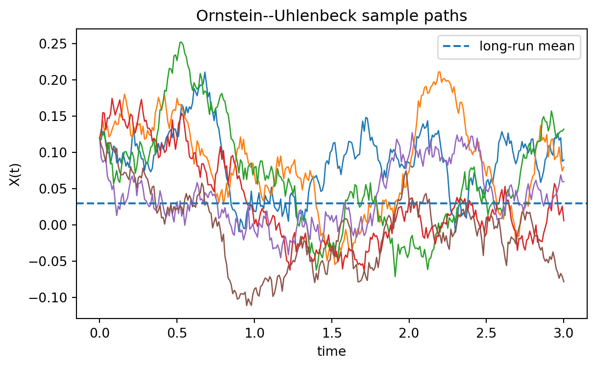
is mean-reverting. If $X_t>\theta$, the drift is negative. If $X_t<\theta$, the drift is positive. Such models are natural for interest rates, spreads, and temporary deviations from equilibrium.
The solution is
$$
X_t=\theta+(X_0-\theta)e^{-\kappa t}+\sigma\int_0^t e^{-\kappa(t-s)}\,dW_s.
$$
Therefore
$$
\mathbb E[X_t]=\theta+(X_0-\theta)e^{-\kappa t},
$$
and
$$
\operatorname{Var}(X_t)=\frac{\sigma^2}{2\kappa}(1-e^{-2\kappa t}).
$$
## 13.6 Interactive Demo: Drift, Volatility, and Sample Paths
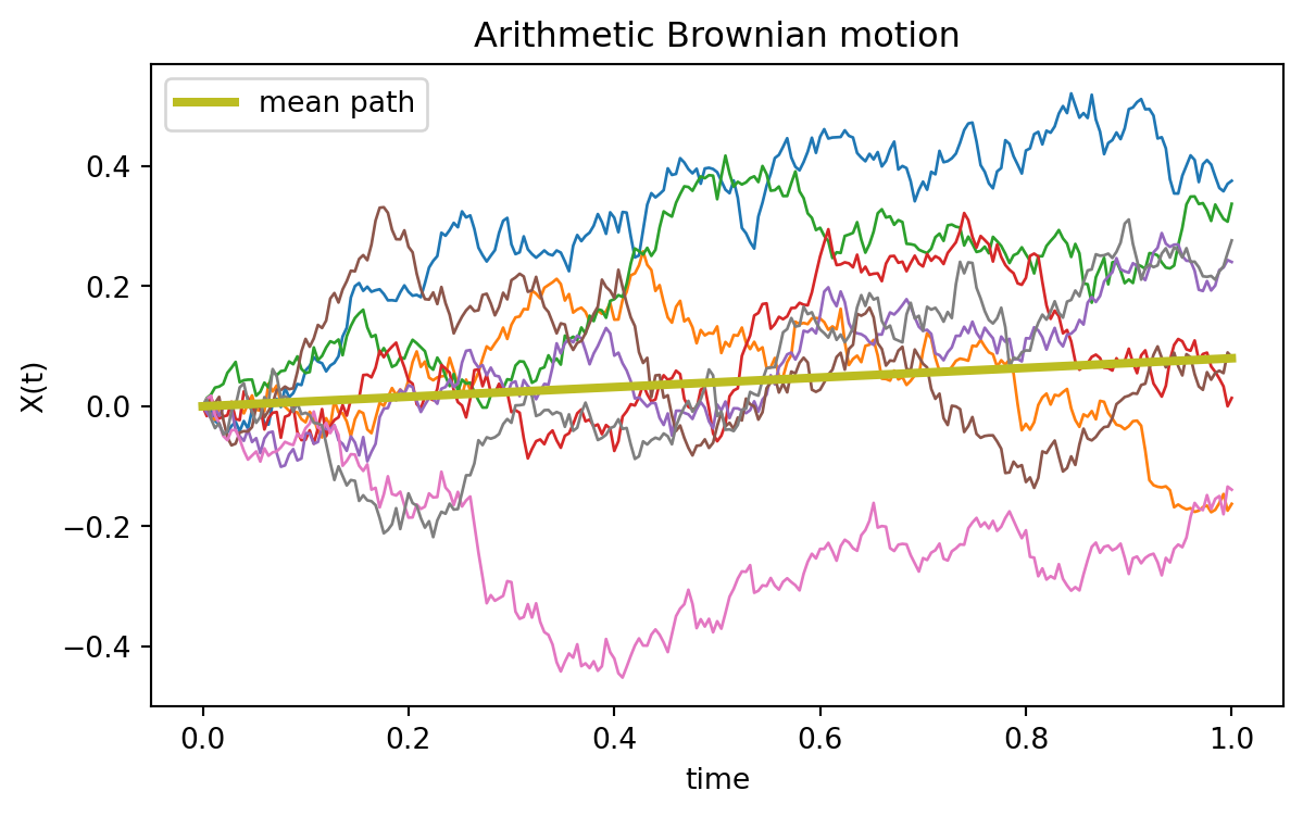
The next activity visualizes how drift and volatility affect simulated SDE paths. The model is arithmetic Brownian motion,
$$
dX_t=\mu\,dt+\sigma\,dW_t.
$$
Changing $\mu$ tilts the cloud of paths. Changing $\sigma$ widens the cloud of paths.
::: {.interactive-card}
### Interactive: Simulated arithmetic Brownian paths
Use the sliders to adjust the drift and volatility. The plot is generated by local Plotly.js.
<div class="mf-controls">
<label for="ch13-abm-mu">Drift $\mu$</label>
<input id="ch13-abm-mu" type="range" min="-0.30" max="0.30" value="0.08" step="0.01">
<span id="ch13-abm-mu-value">0.08</span>
<label for="ch13-abm-sigma">Volatility $\sigma$</label>
<input id="ch13-abm-sigma" type="range" min="0.05" max="0.80" value="0.30" step="0.01">
<span id="ch13-abm-sigma-value">0.30</span>
</div>
<div id="ch13-abm-demo" class="plotly-demo"></div>
<script>
window.mfPlotlyReady(function() {
var el = document.getElementById("ch13-abm-demo");
if (!el) return;
var muSlider = document.getElementById("ch13-abm-mu");
var sigmaSlider = document.getElementById("ch13-abm-sigma");
var muValue = document.getElementById("ch13-abm-mu-value");
var sigmaValue = document.getElementById("ch13-abm-sigma-value");
function normalRandom() {
var u = 0, v = 0;
while (u === 0) u = Math.random();
while (v === 0) v = Math.random();
return Math.sqrt(-2.0 * Math.log(u)) * Math.cos(2.0 * Math.PI * v);
}
function draw() {
var mu = parseFloat(muSlider.value);
var sigma = parseFloat(sigmaSlider.value);
muValue.textContent = mu.toFixed(2);
sigmaValue.textContent = sigma.toFixed(2);
var n = 180;
var T = 1.0;
var dt = T / n;
var t = Array.from({length: n + 1}, function(_, i) { return i * dt; });
var traces = [];
for (var path = 0; path < 25; path++) {
var x = 0.0;
var y = [x];
for (var i = 1; i <= n; i++) {
x += mu * dt + sigma * Math.sqrt(dt) * normalRandom();
y.push(x);
}
traces.push({x: t, y: y, mode: "lines", line: {width: 1}, opacity: 0.55, showlegend: false});
}
traces.push({
x: t,
y: t.map(function(s) { return mu * s; }),
mode: "lines",
name: "mean path",
line: {width: 4}
});
Plotly.react(el, traces, {
title: "Arithmetic Brownian Motion: dX = mu dt + sigma dW",
xaxis: {title: "time"},
yaxis: {title: "X(t)"},
margin: {l: 55, r: 20, t: 50, b: 50}
}, {responsive: true});
}
muSlider.addEventListener("input", draw);
sigmaSlider.addEventListener("input", draw);
draw();
});
</script>
:::
## 13.7 Existence and Uniqueness
An SDE is a mathematical model only if it has a well-defined solution. The most common practical conditions are Lipschitz continuity and linear growth.
::: {.theorem}
### Theorem 13.1: A standard existence and uniqueness theorem
Consider
$$
dX_t=b(t,X_t)\,dt+\sigma(t,X_t)\,dW_t, \qquad X_0=x_0.
$$
Suppose there is a constant $L$ such that, for all $t\in[0,T]$ and all $x,y\in\mathbb R$,
$$
|b(t,x)-b(t,y)|+|\sigma(t,x)-\sigma(t,y)|\le L|x-y|,
$$
and
$$
|b(t,x)|^2+|\sigma(t,x)|^2\le L^2(1+|x|^2).
$$
Then the SDE has a unique strong solution on $[0,T]$.
:::
A strong solution means that $X_t$ is constructed using the given Brownian motion $W_t$ and the given initial condition $X_0$. The word strong refers to the probabilistic construction, not to the size of the solution.
::: {.callout-note}
## Why this theorem matters
In a finance course, students often focus on formulas. But before using a model, one should ask whether the SDE defines a process at all. Linear models such as arithmetic Brownian motion, geometric Brownian motion, and Ornstein--Uhlenbeck dynamics satisfy standard conditions. Some models, such as square-root volatility models, require more careful arguments near zero.
:::
## 13.8 Linear SDEs
Many financial models are linear SDEs. A general one-dimensional linear SDE has the form
$$
dX_t=(a_tX_t+c_t)\,dt+(\alpha_tX_t+\gamma_t)\,dW_t.
$$
Some special cases have explicit solutions. Explicit solutions are valuable because they let us test simulations and understand distributions.
### Constant-Coefficient Additive Noise
If
$$
dX_t=(aX_t+c)\,dt+\sigma\,dW_t,
$$
then an integrating factor gives
$$
X_t=e^{at}X_0+c\int_0^t e^{a(t-s)}\,ds+\sigma\int_0^t e^{a(t-s)}\,dW_s.
$$
If $a\ne0$,
$$
\int_0^t e^{a(t-s)}\,ds=\frac{e^{at}-1}{a}.
$$
The OU model is obtained by taking $a=-\kappa$ and $c=\kappa\theta$.
### Multiplicative Noise
For
$$
dS_t=\mu S_t\,dt+\sigma S_t\,dW_t,
$$
Itô's formula applied to $\log S_t$ gives
$$
d\log S_t=\left(\mu-\frac12\sigma^2\right)dt+\sigma\,dW_t.
$$
Thus
$$
\log S_t=\log S_0+\left(\mu-\frac12\sigma^2\right)t+\sigma W_t.
$$
This explains both the positivity of $S_t$ and the lognormal distribution of prices.
## 13.9 Worked Example: Checking the GBM Solution
We verify that
$$
S_t=S_0\exp\left((\mu-\frac12\sigma^2)t+\sigma W_t\right)
$$
solves
$$
dS_t=\mu S_t\,dt+\sigma S_t\,dW_t.
$$
Let
$$
f(t,w)=S_0\exp\left((\mu-\frac12\sigma^2)t+\sigma w\right).
$$
Then
$$
f_t=(\mu-\frac12\sigma^2)f, \qquad f_w=\sigma f, \qquad f_{ww}=\sigma^2 f.
$$
By Itô's formula,
$$
df(t,W_t)=f_t\,dt+f_w\,dW_t+\frac12 f_{ww}\,dt.
$$
Substitute the derivatives:
$$
dS_t=\left(\mu-\frac12\sigma^2\right)S_t\,dt+\sigma S_t\,dW_t+\frac12\sigma^2S_t\,dt.
$$
The drift terms combine to give
$$
dS_t=\mu S_t\,dt+\sigma S_t\,dW_t.
$$
This proves the claim.
::: {.callout-important}
The correction $-\frac12\sigma^2$ in the exponent is not optional. Without it, applying Itô's formula would produce the wrong drift.
:::
## 13.10 Euler--Maruyama Simulation
For most SDEs, exact simulation is not available. The simplest numerical method is Euler--Maruyama.
Suppose
$$
dX_t=b(t,X_t)\,dt+\sigma(t,X_t)\,dW_t.
$$
Choose a time grid
$$
0=t_0<t_1<\cdots<t_N=T,
$$
with step size $\Delta t=T/N$. Let
$$
\Delta W_n=W_{t_{n+1}}-W_{t_n}=\sqrt{\Delta t}Z_n,
$$
where $Z_n\sim N(0,1)$ independently. The Euler--Maruyama approximation is
$$
X_{n+1}=X_n+b(t_n,X_n)\Delta t+\sigma(t_n,X_n)\Delta W_n.
$$
This method is a direct discretization of the integral equation. The drift is frozen at the left endpoint, and the diffusion coefficient is frozen at the left endpoint.
::: {.definition}
### Definition 13.2: Strong and weak numerical error
Let $X_T$ be the true value and $X_T^{\Delta t}$ be a numerical approximation.
The strong error measures pathwise accuracy:
$$
\mathbb E[|X_T-X_T^{\Delta t}|].
$$
The weak error measures expectation accuracy for test functions $g$:
$$
|\mathbb E[g(X_T)]-\mathbb E[g(X_T^{\Delta t})]|.
$$
:::
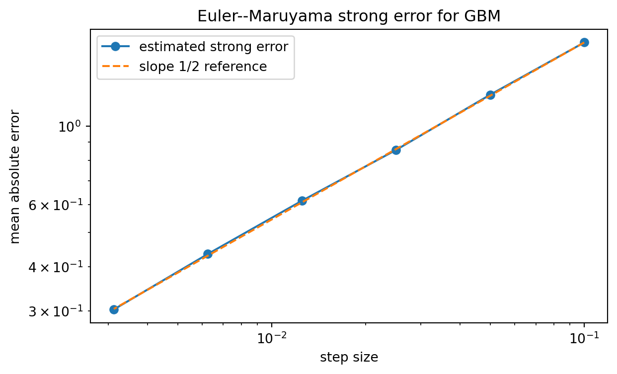
For many smooth SDEs, Euler--Maruyama has strong order $1/2$ and weak order $1$. Informally,
$$
\text{strong error} \approx C\Delta t^{1/2},
$$
while
$$
\text{weak error} \approx C\Delta t.
$$
In finance, weak error is often important for pricing expectations, while strong error matters for pathwise hedging and scenario analysis.
## 13.11 Python Example: Arithmetic Brownian Motion
```{python}
#| label: ch13-python-abm
#| fig-cap: "Simulated arithmetic Brownian motion paths."
import numpy as np
import matplotlib.pyplot as plt

rng = np.random.default_rng(1301)

T = 1.0
N = 250
M = 8
mu = 0.08
sigma = 0.30
x0 = 0.0

dt = T / N
time = np.linspace(0, T, N + 1)
Z = rng.normal(size=(M, N))
dW = np.sqrt(dt) * Z

X = np.zeros((M, N + 1))
X[:, 0] = x0
for n in range(N):
    X[:, n + 1] = X[:, n] + mu * dt + sigma * dW[:, n]

plt.figure(figsize=(7, 4))
for m in range(M):
    plt.plot(time, X[m], linewidth=1)
plt.plot(time, x0 + mu * time, linewidth=3, label="mean path")
plt.xlabel("time")
plt.ylabel("X(t)")
plt.title("Arithmetic Brownian motion")
plt.legend()
plt.show()
```
At the final time,
$$
X_T\sim N(x_0+\mu T,\sigma^2T).
$$
The following code checks the simulated mean and variance.
```{python}
#| label: ch13-python-abm-moments
rng = np.random.default_rng(1302)

T = 1.0
N = 250
M = 50_000
mu = 0.08
sigma = 0.30
x0 = 0.0

dt = T / N
Z = rng.normal(size=(M, N))
X_T = x0 + mu * T + sigma * np.sqrt(dt) * Z.sum(axis=1)

print("Simulated mean:", X_T.mean())
print("Theoretical mean:", x0 + mu * T)
print("Simulated variance:", X_T.var(ddof=1))
print("Theoretical variance:", sigma**2 * T)
```
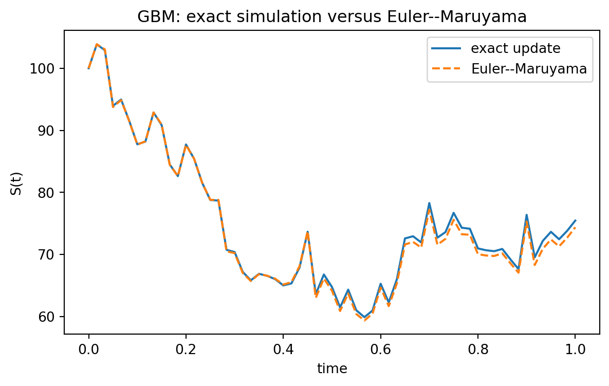
## 13.12 Python Example: Exact GBM Versus Euler--Maruyama
For geometric Brownian motion, exact simulation is available:
$$
S_{t_{n+1}}=S_{t_n}\exp\left((\mu-\frac12\sigma^2)\Delta t+\sigma\Delta W_n\right).
$$
Euler--Maruyama gives
$$
S_{n+1}=S_n+\mu S_n\Delta t+\sigma S_n\Delta W_n.
$$
The exact update preserves positivity. Euler--Maruyama may produce negative values when the step size is too large or volatility is too high.
```{python}
#| label: ch13-python-gbm-exact-euler
#| fig-cap: "Exact and Euler simulation of the same GBM Brownian path."
import numpy as np
import matplotlib.pyplot as plt

rng = np.random.default_rng(1303)

S0 = 100.0
mu = 0.10
sigma = 0.35
T = 1.0
N = 60

dt = T / N
time = np.linspace(0, T, N + 1)
dW = np.sqrt(dt) * rng.normal(size=N)

S_exact = np.empty(N + 1)
S_euler = np.empty(N + 1)
S_exact[0] = S0
S_euler[0] = S0

for n in range(N):
    S_exact[n + 1] = S_exact[n] * np.exp((mu - 0.5 * sigma**2) * dt + sigma * dW[n])
    S_euler[n + 1] = S_euler[n] + mu * S_euler[n] * dt + sigma * S_euler[n] * dW[n]

plt.figure(figsize=(7, 4))
plt.plot(time, S_exact, label="exact update")
plt.plot(time, S_euler, linestyle="--", label="Euler--Maruyama")
plt.xlabel("time")
plt.ylabel("S(t)")
plt.title("GBM: exact simulation versus Euler--Maruyama")
plt.legend()
plt.show()

print("Final exact value:", S_exact[-1])
print("Final Euler value:", S_euler[-1])
```
## 13.13 Interactive Demo: Mean Reversion
The Ornstein--Uhlenbeck model
$$
dX_t=\kappa(\theta-X_t)\,dt+\sigma\,dW_t
$$
has a parameter $\kappa$ controlling the speed of mean reversion. Larger $\kappa$ pulls paths toward $\theta$ more quickly.
::: {.interactive-card}
### Interactive: Ornstein--Uhlenbeck mean reversion
<div class="mf-controls">
<label for="ch13-ou-kappa">Mean-reversion speed $\kappa$</label>
<input id="ch13-ou-kappa" type="range" min="0.10" max="5.00" value="1.50" step="0.10">
<span id="ch13-ou-kappa-value">1.50</span>
<label for="ch13-ou-sigma">Volatility $\sigma$</label>
<input id="ch13-ou-sigma" type="range" min="0.05" max="0.80" value="0.25" step="0.01">
<span id="ch13-ou-sigma-value">0.25</span>
</div>
<div id="ch13-ou-demo" class="plotly-demo"></div>
<script>
window.mfPlotlyReady(function() {
var el = document.getElementById("ch13-ou-demo");
if (!el) return;
var kappaSlider = document.getElementById("ch13-ou-kappa");
var sigmaSlider = document.getElementById("ch13-ou-sigma");
var kappaValue = document.getElementById("ch13-ou-kappa-value");
var sigmaValue = document.getElementById("ch13-ou-sigma-value");
function normalRandom() {
var u = 0, v = 0;
while (u === 0) u = Math.random();
while (v === 0) v = Math.random();
return Math.sqrt(-2.0 * Math.log(u)) * Math.sin(2.0 * Math.PI * v);
}
function draw() {
var kappa = parseFloat(kappaSlider.value);
var sigma = parseFloat(sigmaSlider.value);
var theta = 0.03;
var x0 = 0.12;
kappaValue.textContent = kappa.toFixed(2);
sigmaValue.textContent = sigma.toFixed(2);
var n = 240;
var T = 2.0;
var dt = T / n;
var t = Array.from({length: n + 1}, function(_, i) { return i * dt; });
var traces = [];
for (var path = 0; path < 25; path++) {
var x = x0;
var y = [x];
for (var i = 1; i <= n; i++) {
x += kappa * (theta - x) * dt + sigma * Math.sqrt(dt) * normalRandom();
y.push(x);
}
traces.push({x: t, y: y, mode: "lines", line: {width: 1}, opacity: 0.55, showlegend: false});
}
traces.push({
x: t,
y: t.map(function(s) { return theta + (x0 - theta) * Math.exp(-kappa * s); }),
mode: "lines",
name: "conditional mean",
line: {width: 4}
});
traces.push({
x: t,
y: t.map(function() { return theta; }),
mode: "lines",
name: "long-run mean",
line: {width: 2, dash: "dot"}
});
Plotly.react(el, traces, {
title: "Ornstein--Uhlenbeck SDE: mean reversion",
xaxis: {title: "time"},
yaxis: {title: "X(t)"},
margin: {l: 55, r: 20, t: 50, b: 50}
}, {responsive: true});
}
kappaSlider.addEventListener("input", draw);
sigmaSlider.addEventListener("input", draw);
draw();
});
</script>
:::
## 13.14 Python Example: Ornstein--Uhlenbeck Simulation
The exact OU conditional distribution is normal:
$$
X_{t+\Delta t}\mid X_t=x
\sim
N\left(\theta+(x-\theta)e^{-\kappa\Delta t},\frac{\sigma^2}{2\kappa}(1-e^{-2\kappa\Delta t})\right).
$$
This gives an exact simulation scheme. It is often better than Euler--Maruyama for mean-reverting models.
```{python}
#| label: ch13-python-ou-exact
#| fig-cap: "Exact simulation of an Ornstein--Uhlenbeck process."
import numpy as np
import matplotlib.pyplot as plt

rng = np.random.default_rng(1304)

kappa = 1.8
theta = 0.03
sigma = 0.12
x0 = 0.12
T = 3.0
N = 300
M = 6

dt = T / N
time = np.linspace(0, T, N + 1)
mean_factor = np.exp(-kappa * dt)
step_sd = np.sqrt(sigma**2 / (2 * kappa) * (1 - np.exp(-2 * kappa * dt)))

X = np.empty((M, N + 1))
X[:, 0] = x0
for n in range(N):
    conditional_mean = theta + (X[:, n] - theta) * mean_factor
    X[:, n + 1] = conditional_mean + step_sd * rng.normal(size=M)

plt.figure(figsize=(7, 4))
for m in range(M):
    plt.plot(time, X[m], linewidth=1)
plt.axhline(theta, linestyle="--", label="long-run mean")
plt.xlabel("time")
plt.ylabel("X(t)")
plt.title("Ornstein--Uhlenbeck sample paths")
plt.legend()
plt.show()
```
## 13.15 Generators and PDE Connection
For the SDE
$$
dX_t=b(t,X_t)\,dt+\sigma(t,X_t)\,dW_t,
$$
Itô's formula gives, for a smooth function $f(t,x)$,
$$
df(t,X_t)
=
\left(f_t+b f_x+\frac12\sigma^2 f_{xx}\right)(t,X_t)\,dt
+
\sigma(t,X_t)f_x(t,X_t)\,dW_t.
$$
The spatial operator
$$
L f(x)=b(x)f'(x)+\frac12\sigma^2(x)f''(x)
$$
is called the infinitesimal generator for a time-homogeneous diffusion.
If
$$
u(t,x)=\mathbb E[g(X_T)\mid X_t=x],
$$
then $u$ typically solves the backward Kolmogorov equation
$$
u_t(t,x)+L u(t,x)=0, \qquad u(T,x)=g(x).
$$
This is a major bridge between SDEs, partial differential equations, and derivative pricing.
::: {.callout-note}
The Black--Scholes PDE in Chapter 15 is a financial version of this idea. Hedging changes the drift condition, but the second-order term comes from the diffusion variance in the SDE.
:::
## 13.16 Physical Measure Versus Risk-Neutral Measure
A financial SDE must specify the probability measure. Under a physical measure $\mathbb P$, one might write
$$
dS_t=\mu S_t\,dt+\sigma S_t\,dW_t^{\mathbb P}.
$$
Under a risk-neutral measure $\mathbb Q$, a non-dividend-paying stock in a Black--Scholes market satisfies
$$
dS_t=rS_t\,dt+\sigma S_t\,dW_t^{\mathbb Q}.
$$
The volatility coefficient is the same in this simple model, but the drift changes from $\mu$ to $r$. The measure change is studied in Chapter 17.
The distinction matters because simulation for risk estimation often uses $\mathbb P$, while derivative pricing often uses $\mathbb Q$.
::: {.warning}
A common mistake is to estimate a historical drift $\mu$ from data and then insert it directly into an option-pricing formula. In no-arbitrage pricing, the drift used for pricing is determined by the pricing measure, not by the historical mean return.
:::
## 13.17 Python Example: Pricing an Expectation by Monte Carlo
Consider a European call payoff under the risk-neutral GBM model
$$
dS_t=rS_t\,dt+\sigma S_t\,dW_t^{\mathbb Q}.
$$
The no-arbitrage price is
$$
C_0=e^{-rT}\mathbb E^{\mathbb Q}[(S_T-K)^+].
$$
The following code estimates the expectation by exact simulation of $S_T$.
```{python}
#| label: ch13-python-monte-carlo-call
import numpy as np
from math import exp, log, sqrt, erf

rng = np.random.default_rng(1305)

S0 = 100.0
K = 105.0
r = 0.04
sigma = 0.25
T = 1.0
M = 200_000

Z = rng.normal(size=M)
S_T = S0 * np.exp((r - 0.5 * sigma**2) * T + sigma * np.sqrt(T) * Z)
payoff = np.maximum(S_T - K, 0.0)
mc_price = np.exp(-r * T) * payoff.mean()
mc_se = np.exp(-r * T) * payoff.std(ddof=1) / np.sqrt(M)

def normal_cdf(x):
    return 0.5 * (1.0 + erf(x / sqrt(2.0)))

d1 = (log(S0 / K) + (r + 0.5 * sigma**2) * T) / (sigma * sqrt(T))
d2 = d1 - sigma * sqrt(T)
bs_price = S0 * normal_cdf(d1) - K * exp(-r * T) * normal_cdf(d2)

print("Monte Carlo price:", mc_price)
print("Monte Carlo standard error:", mc_se)
print("Black--Scholes price:", bs_price)
```
This example uses an SDE simulation, but it also previews risk-neutral pricing and the Black--Scholes formula.
## 13.18 Python Example: Strong Error of Euler--Maruyama for GBM
To estimate strong error, simulate the exact and approximate solutions using the same Brownian path. For GBM, this is possible because the exact solution is known.
```{python}
#| label: ch13-python-strong-error
#| fig-cap: "Strong error of Euler--Maruyama for GBM on a log-log scale."
import numpy as np
import matplotlib.pyplot as plt

rng = np.random.default_rng(1306)

S0 = 100.0
mu = 0.08
sigma = 0.30
T = 1.0
M = 20_000
steps_list = np.array([10, 20, 40, 80, 160, 320])
errors = []

for N in steps_list:
    dt = T / N
    Z = rng.normal(size=(M, N))
    dW = np.sqrt(dt) * Z
    W_T = dW.sum(axis=1)
    S_exact_T = S0 * np.exp((mu - 0.5 * sigma**2) * T + sigma * W_T)

    S_euler = np.full(M, S0)
    for n in range(N):
        S_euler = S_euler + mu * S_euler * dt + sigma * S_euler * dW[:, n]

    errors.append(np.mean(np.abs(S_exact_T - S_euler)))

errors = np.array(errors)

plt.figure(figsize=(7, 4))
plt.loglog(T / steps_list, errors, marker="o", label="estimated strong error")
plt.loglog(T / steps_list, errors[0] * ((T / steps_list) / (T / steps_list[0]))**0.5,
           linestyle="--", label="slope 1/2 reference")
plt.xlabel("step size")
plt.ylabel("mean absolute error")
plt.title("Euler--Maruyama strong error for GBM")
plt.legend()
plt.show()

for N, err in zip(steps_list, errors):
    print(f"N={N:3d}, dt={T/N:.5f}, strong error={err:.5f}")
```
The plot should show an approximate slope of $1/2$ on a log-log scale. Monte Carlo randomness and finite sample size make the slope imperfect.
## 13.19 Modeling Choices and Common Financial SDEs
The following table summarizes several important SDE models.
| Model | SDE | Typical use | Key feature |
|---|---|---|---|
| Arithmetic Brownian motion | $dX_t=\mu\,dt+\sigma\,dW_t$ | additive changes, spreads | normal values; can be negative |
| Geometric Brownian motion | $dS_t=\mu S_t\,dt+\sigma S_t\,dW_t$ | stock prices | positive; lognormal |
| Ornstein--Uhlenbeck | $dX_t=\kappa(\theta-X_t)\,dt+\sigma\,dW_t$ | rates, spreads, signals | mean reversion |
| Vasicek short rate | $dr_t=a(b-r_t)\,dt+\sigma\,dW_t$ | interest rates | Gaussian rates; may be negative |
| CIR short rate | $dr_t=a(b-r_t)\,dt+\sigma\sqrt{r_t}\,dW_t$ | interest rates, variance | nonnegative under conditions |
| Heston variance | $dv_t=\kappa(\theta-v_t)\,dt+\xi\sqrt{v_t}\,dW_t$ | stochastic volatility | random volatility |
Each model encodes assumptions. For example, GBM assumes constant volatility and continuous paths. A jump model relaxes continuity. A stochastic volatility model relaxes constant volatility. A regime-switching model relaxes constant parameters.
## 13.20 AI-Assisted Learning Components
AI tools can help students test explanations, debug simulations, and compare models. They should not replace the mathematical definitions.
::: {.callout-tip}
## AI prompt: Explain an SDE carefully
Ask an AI assistant:
> Explain why $dX_t=b(t,X_t)dt+\sigma(t,X_t)dW_t$ must be interpreted as an integral equation. Give one financial reason why adaptedness matters. Avoid saying that Brownian motion has an ordinary derivative.
Then check whether the response explicitly mentions the Itô integral and the filtration.
:::
::: {.callout-tip}
## AI prompt: Audit Euler--Maruyama code
Give an AI assistant a simulation code block and ask:
> Check whether this code uses independent normal increments with variance $\Delta t$, whether the drift and diffusion are evaluated at the left endpoint, and whether the random seed makes the simulation reproducible.
Then verify the answer manually.
:::
::: {.callout-tip}
## AI prompt: Model critique
Ask:
> I am modeling a stock price by arithmetic Brownian motion. What mathematical and financial problems can occur? Compare with geometric Brownian motion.
A good answer should mention positivity, additive versus multiplicative shocks, normal versus lognormal prices, and the limitations of both models.
:::
## 13.21 Common Mistakes
1. **Treating $dW_t/dt$ as a function.** Brownian motion is not differentiable.
2. **Forgetting the integral form.** An SDE is defined by an ordinary integral plus an Itô integral.
3. **Ignoring adaptedness.** Financial strategies cannot use future Brownian increments.
4. **Confusing drift and volatility.** Drift affects local conditional mean; volatility affects local conditional variance.
5. **Confusing $\mathbb P$ and $\mathbb Q$.** Historical simulation and risk-neutral pricing use different measures.
6. **Using Euler--Maruyama when exact simulation is available.** For GBM and OU models, exact schemes are often preferable.
7. **Assuming Euler preserves constraints.** Euler simulation may make a positive process negative.
8. **Overinterpreting simulated paths.** A few paths show behavior, not proof of a distributional claim.
## 13.22 Exercises
### Conceptual Exercises
1. Explain why the SDE notation $dX_t=b(t,X_t)dt+\sigma(t,X_t)dW_t$ is shorthand for an integral equation.
2. In financial terms, what does adaptedness mean?
3. Explain the difference between drift and volatility using conditional mean and conditional variance.
4. Why is arithmetic Brownian motion usually inappropriate for stock prices?
5. Why is geometric Brownian motion positive?
6. In the OU model, explain the roles of $\kappa$, $\theta$, and $\sigma$.
### Mathematical Exercises
7. Show that arithmetic Brownian motion satisfies
$$
\mathbb E[X_t]=x_0+\mu t
$$
and
$$
\operatorname{Var}(X_t)=\sigma^2t.
$$
8. Use Itô's formula to derive the solution of geometric Brownian motion.
9. Derive the mean and variance of the OU process from its explicit solution.
10. For the SDE
$$
dX_t=aX_t\,dt+\sigma\,dW_t,
$$
derive the explicit solution using an integrating factor.
11. Let
$$
L f(x)=b(x)f'(x)+\frac12\sigma^2(x)f''(x).
$$
Compute $L f$ when $f(x)=x$, $f(x)=x^2$, and $f(x)=e^{ux}$.
### Computational Exercises
12. Simulate arithmetic Brownian motion for different values of $\mu$ and $\sigma$. Compare empirical mean and variance with theory.
13. Simulate GBM using both exact updates and Euler--Maruyama. Count how often Euler produces negative values for large $\sigma$ and large $\Delta t$.
14. Simulate OU paths for different $\kappa$. Explain how the speed of mean reversion changes.
15. Estimate the strong error of Euler--Maruyama for GBM and fit a line on a log-log plot.
16. Use Monte Carlo simulation under the risk-neutral GBM model to estimate a European put price.
### AI-Assisted Exercises
17. Ask an AI assistant to explain the difference between an ODE and an SDE. Identify one sentence that is mathematically precise and one sentence that needs improvement.
18. Ask an AI assistant to generate Euler--Maruyama code for GBM. Audit whether it uses $\sqrt{\Delta t}Z_n$ correctly.
19. Ask an AI assistant to compare GBM and OU models for financial data. Rewrite the answer in precise mathematical language.
20. Ask an AI assistant why option pricing uses a risk-neutral drift. Save the response and mark which claims will be justified only after Chapter 17.
## 13.23 Chapter Summary
An SDE describes a stochastic process through a local drift term and a Brownian diffusion term. The rigorous meaning is an integral equation involving an ordinary integral and an Itô integral. Drift controls local conditional mean, while the diffusion coefficient controls local conditional variance. Existence and uniqueness results ensure that the model is mathematically well defined. Linear SDEs such as arithmetic Brownian motion, geometric Brownian motion, and Ornstein--Uhlenbeck dynamics provide the basic examples for financial modeling. Euler--Maruyama gives a practical simulation method, but exact simulation should be used when available. The chapter also introduced the generator viewpoint and prepared the transition to continuous-time asset pricing.