---
title: "Chapter 10. Brownian Motion"
---
::: {.chapter-objectives}
## Learning Goals
By the end of this chapter, students should be able to:
- explain why Brownian motion is the continuous-time limit of scaled random walks;
- state the defining properties of standard Brownian motion;
- compute finite-dimensional distributions, means, variances, covariances, and correlations of Brownian motion;
- interpret Brownian motion with respect to a filtration and financial information flow;
- distinguish ordinary variation from quadratic variation;
- prove and use the martingale properties of $W_t$, $W_t^2-t$, and exponential Brownian martingales;
- simulate Brownian paths and Brownian increments in Python;
- understand why Brownian motion is continuous but nowhere classically differentiable;
- connect Brownian motion to asset-price modeling, stochastic calculus, and later chapters on Itô integration and Black--Scholes theory;
- use AI tools to audit Brownian-motion simulations, check scaling arguments, and critique financial modeling assumptions.
:::
::: {.hero-box}
Brownian motion is the basic random motion of continuous-time mathematical finance. It is the limiting object behind many repeated small shocks. It has continuous paths, independent Gaussian increments, and quadratic variation equal to time.
The simplest slogan is:
$$
W_t-W_s \sim N(0,t-s),
\qquad 0\le s<t.
$$
The deeper message is that Brownian motion behaves like a random function whose infinitesimal increment satisfies the symbolic rules
$$
\mathbb E[dW_t]=0,
\qquad
(dW_t)^2=dt.
$$
These rules are not ordinary calculus rules. They are the entrance to stochastic calculus.
:::
## 10.1 Why Brownian Motion Appears in Finance
Financial prices move because many small pieces of information arrive over time. No single piece may dominate, but the aggregate effect can produce noisy fluctuations. This is the same mathematical idea behind the central limit theorem: sums of many small, weakly comparable shocks often look approximately Gaussian after suitable scaling.
In discrete time, a simple model for accumulated noise is a random walk
$$
S_n=X_1+X_2+\cdots+X_n,
$$
where $X_1,X_2,\ldots$ are independent shocks with
$$
\mathbb E[X_i]=0,
\qquad
\operatorname{Var}(X_i)=1.
$$
If time is rescaled so that $n$ steps occur in one unit of time, the natural continuous-time interpolation is approximately
$$
W_t^{(n)}=\frac{1}{\sqrt n}S_{\lfloor nt\rfloor}.
$$
The factor $1/\sqrt n$ is essential. Since the variance of $S_{\lfloor nt\rfloor}$ is approximately $nt$, the variance of $W_t^{(n)}$ is approximately
$$
\operatorname{Var}(W_t^{(n)})
=
\frac{1}{n}\operatorname{Var}(S_{\lfloor nt\rfloor})
\approx t.
$$
Thus the limiting process should have variance growing linearly in time. Brownian motion is exactly the continuous-time process with this scaling property and Gaussian independent increments.
::: {.callout-note}
## Financial interpretation
Brownian motion is not a model for the stock price itself. A stock price should usually remain positive. Instead, Brownian motion is a model for the cumulative random shock driving log prices, interest rates, volatility, or other state variables.
:::
## 10.2 From Random Walks to a Continuous-Time Limit
Let $X_1,X_2,\ldots$ be independent random variables satisfying
$$
\mathbb P(X_i=1)=\mathbb P(X_i=-1)=\frac12.
$$
Define the scaled random walk
$$
W_t^{(n)}=\frac{1}{\sqrt n}\sum_{k=1}^{\lfloor nt\rfloor}X_k.
$$
For a fixed time $t$, the central limit theorem gives
$$
W_t^{(n)}
\Rightarrow
N(0,t)
$$
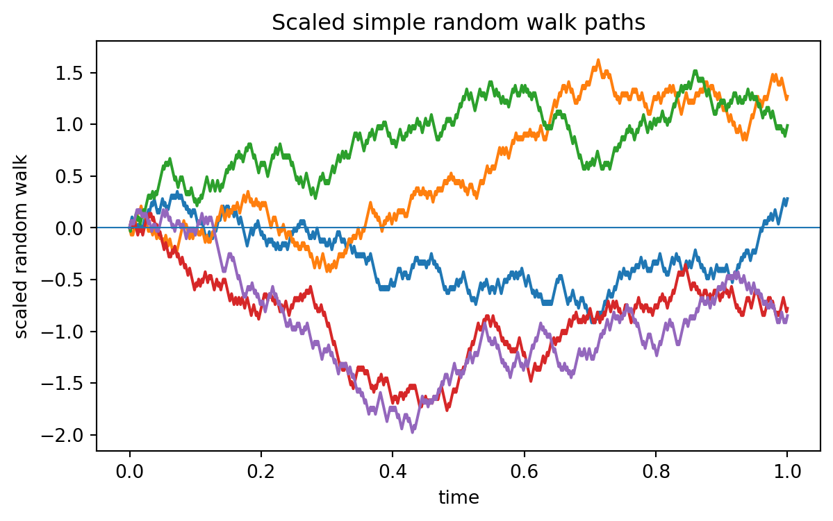
as $n\to\infty$. More generally, the joint distribution at finitely many time points converges to the joint distribution of Brownian motion. A precise process-level convergence theorem is called Donsker's invariance principle.
For this book, the key idea is more important than the full theorem:
$$
\text{many small independent shocks}
\quad\Longrightarrow\quad
\text{Brownian noise}.
$$
::: {.example}
### Example 10.1: Scaling of a random walk
Suppose one step has variance $1$. After $n$ steps, the variance is $n$. If we divide the random walk by $\sqrt n$, then the variance after $n$ steps becomes $1$.
At time $t$, there are approximately $nt$ steps. Therefore
$$
\operatorname{Var}\left(\frac{S_{\lfloor nt\rfloor}}{\sqrt n}\right)
\approx
\frac{nt}{n}=t.
$$
This explains why Brownian motion satisfies $\operatorname{Var}(W_t)=t$.
:::
```{python}
#| label: py-ch10-random-walk-scaling
#| fig-cap: "Scaled random walks begin to resemble Brownian motion."
import numpy as np
import matplotlib.pyplot as plt

rng = np.random.default_rng(7243)
T = 1.0
n = 800
m_paths = 5

time = np.linspace(0, T, n + 1)

plt.figure(figsize=(7, 4))
for _ in range(m_paths):
    steps = rng.choice([-1, 1], size=n)
    path = np.concatenate([[0], np.cumsum(steps) / np.sqrt(n)])
    plt.plot(time, path, linewidth=1.5)

plt.axhline(0, linewidth=0.8)
plt.xlabel("time")
plt.ylabel("scaled random walk")
plt.title("Scaled simple random walk paths")
plt.show()
```
## 10.3 Definition of Brownian Motion
We now state the mathematical definition.
::: {.definition}
### Definition 10.1: Standard Brownian motion
A stochastic process $(W_t)_{t\ge 0}$ is a standard Brownian motion if:
1. $W_0=0$ almost surely;
2. $W_t-W_s\sim N(0,t-s)$ for all $0\le s<t$;
3. increments over disjoint time intervals are independent;
4. the sample paths $t\mapsto W_t(\omega)$ are continuous almost surely.
:::
The first three conditions describe the finite-dimensional distributions. The fourth condition says that the random path has no jumps.
The notation $W_t$ is standard. Some books use $B_t$. In finance, $W_t$ is common because it is interpreted as a Wiener process.
::: {.warning}
Brownian paths are continuous, but they are not smooth. A Brownian path is almost surely nowhere differentiable. Thus Brownian motion is not a random curve in the ordinary calculus sense.
:::
## 10.4 Gaussian Increments and Basic Distributions
For standard Brownian motion,
$$
W_t\sim N(0,t).
$$
Therefore
$$
\mathbb E[W_t]=0,
\qquad
\operatorname{Var}(W_t)=t.
$$
If $0\le s<t$, then
$$
W_t=W_s+(W_t-W_s),
$$
where $W_s$ and $W_t-W_s$ are independent. Hence
$$
\operatorname{Var}(W_t)=\operatorname{Var}(W_s)+\operatorname{Var}(W_t-W_s)=s+(t-s)=t.
$$
The increment density is
$$
f_{W_t-W_s}(x)
=
\frac{1}{\sqrt{2\pi(t-s)}}\exp\left(-\frac{x^2}{2(t-s)}\right).
$$
::: {.example}
### Example 10.2: Probability of a Brownian increment
Let $W$ be standard Brownian motion. Then
$$
W_{0.75}-W_{0.25}\sim N(0,0.5).
$$
Therefore
$$
\mathbb P(W_{0.75}-W_{0.25}>1)
=
1-\Phi\left(\frac{1}{\sqrt{0.5}}\right).
$$
The probability is small because a move of size $1$ over a time interval of length $0.5$ is about $1.414$ standard deviations.
:::
```{python}
#| label: py-ch10-increment-probability
# Brownian increment probability using scipy if available, otherwise using math.erf.
import math

variance = 0.5
z = 1 / math.sqrt(variance)
Phi = lambda x: 0.5 * (1 + math.erf(x / math.sqrt(2)))
probability = 1 - Phi(z)

print("z-score:", round(z, 4))
print("P(W_0.75 - W_0.25 > 1):", round(probability, 6))
```
## 10.5 Covariance Structure
Brownian motion is a Gaussian process. This means that for any finite set of times
$$
0\le t_1<t_2<\cdots<t_m,
$$
the random vector
$$
(W_{t_1},W_{t_2},\ldots,W_{t_m})
$$
has a multivariate normal distribution.
The covariance function is especially simple:
$$
\operatorname{Cov}(W_s,W_t)=\min(s,t).
$$
::: {.proof}
Assume $0\le s\le t$. Then
$$
W_t=W_s+(W_t-W_s),
$$
where $W_t-W_s$ is independent of $W_s$. Thus
$$
\operatorname{Cov}(W_s,W_t)
=
\operatorname{Cov}(W_s,W_s)+\operatorname{Cov}(W_s,W_t-W_s)
=s+0=s.
$$
Since $s=\min(s,t)$ in this case, the formula follows. The case $t\le s$ is symmetric.
:::
The correlation is therefore
$$
\operatorname{Corr}(W_s,W_t)
=
\frac{\min(s,t)}{\sqrt{st}}.
$$
If $s<t$, this becomes
$$
\operatorname{Corr}(W_s,W_t)=\sqrt{\frac{s}{t}}.
$$
Thus values of Brownian motion at nearby times are highly correlated, even though nonoverlapping increments are independent.
::: {.callout-note}
## Important distinction
Brownian levels are correlated:
$$
W_s \text{ and } W_t \text{ are usually correlated.}
$$
Brownian increments over disjoint intervals are independent:
$$
W_b-W_a \text{ and } W_d-W_c \text{ are independent if } [a,b]\cap[c,d]=\varnothing.
$$
:::
```{python}
#| label: py-ch10-covariance-matrix
import numpy as np

# Brownian covariance matrix at selected times.
times = np.array([0.25, 0.50, 1.00, 2.00])
Sigma = np.minimum.outer(times, times)

print("Times:", times)
print("Brownian covariance matrix:")
print(np.round(Sigma, 3))
```
## 10.6 Brownian Motion as a Martingale
Let $(\mathcal F_t)_{t\ge 0}$ be the natural filtration generated by Brownian motion:
$$
\mathcal F_t=\sigma(W_s:0\le s\le t).
$$
This represents the information contained in the Brownian path up to time $t$.
Brownian motion is adapted to its natural filtration because $W_t$ is known at time $t$. It is also a martingale.
::: {.theorem}
### Theorem 10.1: Brownian motion is a martingale
For $0\le s<t$,
$$
\mathbb E[W_t\mid \mathcal F_s]=W_s.
$$
:::
::: {.proof}
Write
$$
W_t=W_s+(W_t-W_s).
$$
The increment $W_t-W_s$ is independent of $\mathcal F_s$ and has mean zero. Therefore
$$
\mathbb E[W_t\mid \mathcal F_s]
=
\mathbb E[W_s+W_t-W_s\mid \mathcal F_s]
=W_s+\mathbb E[W_t-W_s]
=W_s.
$$
:::
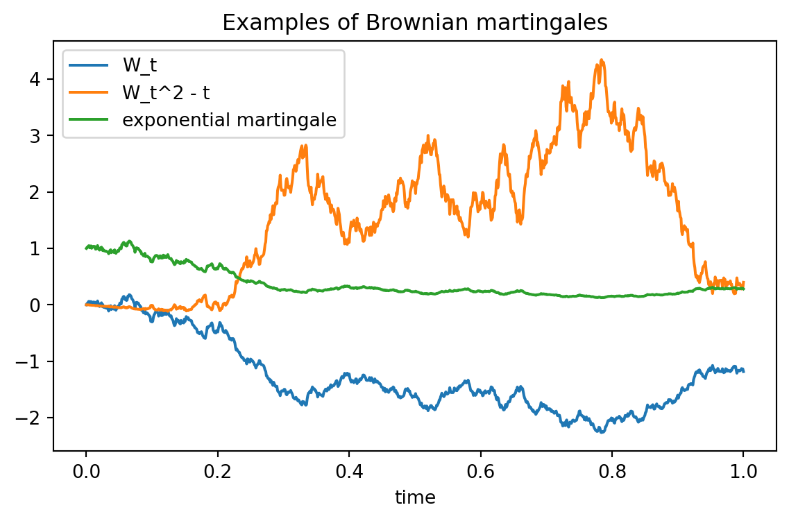
Brownian motion also generates other martingales.
::: {.theorem}
### Theorem 10.2: Two standard Brownian martingales
For standard Brownian motion,
$$
M_t=W_t^2-t
$$
is a martingale. Also, for any fixed $\theta\in\mathbb R$,
$$
Z_t=\exp\left(\theta W_t-\frac12\theta^2t\right)
$$
is a martingale.
:::
::: {.proof}
For $M_t$, write $W_t=W_s+Y$, where $Y=W_t-W_s\sim N(0,t-s)$ is independent of $\mathcal F_s$. Then
$$
\mathbb E[W_t^2\mid\mathcal F_s]
=
\mathbb E[(W_s+Y)^2\mid\mathcal F_s]
=W_s^2+2W_s\mathbb E[Y]+\mathbb E[Y^2]
=W_s^2+t-s.
$$
Thus
$$
\mathbb E[W_t^2-t\mid\mathcal F_s]
=W_s^2+t-s-t
=W_s^2-s.
$$
For $Z_t$, use the moment-generating function of a normal random variable. Since $Y\sim N(0,t-s)$,
$$
\mathbb E[e^{\theta Y}]=e^{\frac12\theta^2(t-s)}.
$$
Therefore
$$
\mathbb E[Z_t\mid\mathcal F_s]
=
\exp\left(\theta W_s-\frac12\theta^2t\right)
\mathbb E[e^{\theta Y}]
=
\exp\left(\theta W_s-\frac12\theta^2s\right)
=Z_s.
$$
:::
::: {.callout-note}
## Why exponential martingales matter in finance
The exponential Brownian martingale is the mathematical object behind change of measure and Girsanov's theorem. Later, it will be used to move from the physical probability measure $\mathbb P$ to a risk-neutral probability measure $\mathbb Q$.
:::
```{python}
#| label: py-ch10-brownian-martingales
#| fig-cap: "Brownian martingales along simulated paths."
import numpy as np
import matplotlib.pyplot as plt

rng = np.random.default_rng(5110)
T = 1.0
n = 1000
dt = T / n
time = np.linspace(0, T, n + 1)

dW = rng.normal(0.0, np.sqrt(dt), size=n)
W = np.concatenate([[0.0], np.cumsum(dW)])

theta = 0.8
M = W**2 - time
Z = np.exp(theta * W - 0.5 * theta**2 * time)

plt.figure(figsize=(7, 4))
plt.plot(time, W, label="W_t")
plt.plot(time, M, label="W_t^2 - t")
plt.plot(time, Z, label="exponential martingale")
plt.xlabel("time")
plt.title("Examples of Brownian martingales")
plt.legend()
plt.show()
```
## 10.7 Interactive Demo: Brownian Sample Paths
The next interactive visualizes Brownian sample paths. Increasing the number of steps makes the path look more irregular, not smoother in the classical sense. This is one of the important surprises of Brownian motion.
::: {.interactive-card}
### Interactive 10.1: Simulate Brownian paths
Use the sliders to change the time horizon, number of discretization steps, and number of simulated paths.
<div class="mf-controls">
<label for="mf-ch10-paths-T">time horizon $T$</label>
<input id="mf-ch10-paths-T" type="range" min="0.5" max="3" step="0.5" value="1">
<label for="mf-ch10-paths-n">number of steps</label>
<input id="mf-ch10-paths-n" type="range" min="50" max="800" step="50" value="250">
<label for="mf-ch10-paths-m">number of paths</label>
<input id="mf-ch10-paths-m" type="range" min="1" max="12" step="1" value="5">
</div>
<div id="mf-ch10-paths-plot" class="plotly-demo"></div>
<div id="mf-ch10-paths-output" class="mf-output"></div>
<script>
(window.mfPlotlyReady || function(f){ if (document.readyState === "loading") { document.addEventListener("DOMContentLoaded", f); } else { f(); } })(function() {
const TSlider = document.getElementById("mf-ch10-paths-T");
const nSlider = document.getElementById("mf-ch10-paths-n");
const mSlider = document.getElementById("mf-ch10-paths-m");
const plotDiv = document.getElementById("mf-ch10-paths-plot");
const output = document.getElementById("mf-ch10-paths-output");
if (!TSlider || !nSlider || !mSlider || !plotDiv || typeof Plotly === "undefined") return;
function normal01() {
let u = 0, v = 0;
while (u === 0) u = Math.random();
while (v === 0) v = Math.random();
return Math.sqrt(-2 * Math.log(u)) * Math.cos(2 * Math.PI * v);
}
function update() {
const T = Number(TSlider.value);
const n = Number(nSlider.value);
const m = Number(mSlider.value);
const dt = T / n;
const time = Array.from({length: n + 1}, (_, i) => i * dt);
const traces = [];
const terminal = [];
for (let k = 0; k < m; k++) {
let w = 0;
const y = [0];
for (let i = 1; i <= n; i++) {
w += Math.sqrt(dt) * normal01();
y.push(w);
}
terminal.push(w);
traces.push({x: time, y: y, mode: "lines", name: "path " + (k + 1)});
}
Plotly.react(plotDiv, traces, {
title: "Simulated Brownian Motion Paths",
xaxis: {title: "time"},
yaxis: {title: "W_t"},
margin: {l: 55, r: 20, t: 50, b: 50}
}, {responsive: true});
const meanTerminal = terminal.reduce((a, b) => a + b, 0) / terminal.length;
const varianceTerminal = terminal.reduce((a, b) => a + Math.pow(b - meanTerminal, 2), 0) / Math.max(1, terminal.length - 1);
output.innerHTML = `Theoretical distribution: W_T ~ N(0, ${T.toFixed(2)}). ` +
`For these ${m} paths, terminal sample mean is ${meanTerminal.toFixed(3)} and terminal sample variance is ${varianceTerminal.toFixed(3)}.`;
}
[TSlider, nSlider, mSlider].forEach(el => el.addEventListener("input", update));
update();
});
</script>
:::
## 10.8 Quadratic Variation
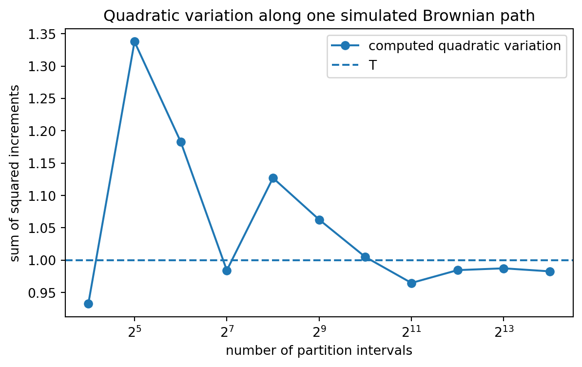
Brownian motion has a surprising path property: its ordinary variation is infinite, but its quadratic variation is finite and equal to elapsed time.
Take a partition of $[0,T]$:
$$
0=t_0<t_1<\cdots<t_n=T.
$$
The quadratic variation along this partition is
$$
\sum_{k=0}^{n-1}(W_{t_{k+1}}-W_{t_k})^2.
$$
For Brownian motion, as the partition gets finer,
$$
\sum_{k=0}^{n-1}(W_{t_{k+1}}-W_{t_k})^2
\to T
$$
in probability, and along many natural sequences of partitions, almost surely.
This fact is the reason stochastic calculus differs from ordinary calculus. In ordinary calculus, if $x(t)$ is a smooth function, then the squared increment is tiny compared with $dt$:
$$
(dx)^2 \approx 0.
$$
For Brownian motion, the squared increment accumulates:
$$
(dW_t)^2=dt.
$$
::: {.proof}
Consider an equally spaced partition with $\Delta t=T/n$. The increments
$$
\Delta W_k=W_{t_{k+1}}-W_{t_k}
$$
are independent and satisfy
$$
\Delta W_k\sim N(0,\Delta t).
$$
Therefore
$$
\mathbb E[(\Delta W_k)^2]=\Delta t.
$$
So
$$
\mathbb E\left[\sum_{k=0}^{n-1}(\Delta W_k)^2\right]
=
\sum_{k=0}^{n-1}\Delta t
=T.
$$
A variance computation shows that the variance of this sum goes to $0$ as $n\to\infty$. Hence the sum converges to $T$ in probability.
:::
```{python}
#| label: py-ch10-quadratic-variation
#| fig-cap: "Quadratic variation of one Brownian path stabilizes near T as the partition is refined."
import numpy as np
import matplotlib.pyplot as plt

rng = np.random.default_rng(6241)
T = 1.0
n_fine = 2**14
dt_fine = T / n_fine

dW_fine = rng.normal(0.0, np.sqrt(dt_fine), size=n_fine)
W_fine = np.concatenate([[0.0], np.cumsum(dW_fine)])

partition_sizes = np.array([2**k for k in range(4, 15)])
qv_values = []
for n in partition_sizes:
    step = n_fine // n
    W_coarse = W_fine[::step]
    qv = np.sum(np.diff(W_coarse)**2)
    qv_values.append(qv)

plt.figure(figsize=(7, 4))
plt.plot(partition_sizes, qv_values, marker="o", label="computed quadratic variation")
plt.axhline(T, linestyle="--", label="T")
plt.xscale("log", base=2)
plt.xlabel("number of partition intervals")
plt.ylabel("sum of squared increments")
plt.title("Quadratic variation along one simulated Brownian path")
plt.legend()
plt.show()

print("Last computed quadratic variation:", round(qv_values[-1], 4))
```
## 10.9 Interactive Demo: Quadratic Variation
The next activity compares the ordinary variation
$$
\sum_k |W_{t_{k+1}}-W_{t_k}|
$$
with the quadratic variation
$$
\sum_k (W_{t_{k+1}}-W_{t_k})^2.
$$
As the partition becomes finer, the quadratic variation stays near $T$, while the ordinary variation tends to grow.
::: {.interactive-card}
### Interactive 10.2: Ordinary variation versus quadratic variation
Move the slider to refine the partition of one simulated Brownian path.
<div class="mf-controls">
<label for="mf-ch10-qv-level">partition level</label>
<input id="mf-ch10-qv-level" type="range" min="4" max="12" step="1" value="7">
</div>
<div id="mf-ch10-qv-plot" class="plotly-demo"></div>
<div id="mf-ch10-qv-output" class="mf-output"></div>
<script>
(window.mfPlotlyReady || function(f){ if (document.readyState === "loading") { document.addEventListener("DOMContentLoaded", f); } else { f(); } })(function() {
const levelSlider = document.getElementById("mf-ch10-qv-level");
const plotDiv = document.getElementById("mf-ch10-qv-plot");
const output = document.getElementById("mf-ch10-qv-output");
if (!levelSlider || !plotDiv || typeof Plotly === "undefined") return;
const T = 1.0;
const nFine = Math.pow(2, 12);
const dt = T / nFine;
const timeFine = Array.from({length: nFine + 1}, (_, i) => i * dt);
// Deterministic pseudo-random generator for stable display.
let seed = 7243;
function rand() {
seed = (1664525 * seed + 1013904223) % 4294967296;
return seed / 4294967296;
}
function normal01() {
let u = 0, v = 0;
while (u === 0) u = rand();
while (v === 0) v = rand();
return Math.sqrt(-2 * Math.log(u)) * Math.cos(2 * Math.PI * v);
}
const WFine = [0];
let w = 0;
for (let i = 1; i <= nFine; i++) {
w += Math.sqrt(dt) * normal01();
WFine.push(w);
}
function update() {
const level = Number(levelSlider.value);
const n = Math.pow(2, level);
const step = nFine / n;
const time = [];
const W = [];
for (let i = 0; i <= n; i++) {
time.push(timeFine[i * step]);
W.push(WFine[i * step]);
}
let ordinary = 0;
let quadratic = 0;
for (let i = 0; i < n; i++) {
const inc = W[i + 1] - W[i];
ordinary += Math.abs(inc);
quadratic += inc * inc;
}
Plotly.react(plotDiv, [
{x: timeFine, y: WFine, mode: "lines", name: "fine Brownian path", line: {width: 1}},
{x: time, y: W, mode: "lines+markers", name: "selected partition"}
], {
title: "Brownian Path with Selected Partition",
xaxis: {title: "time"},
yaxis: {title: "W_t"},
margin: {l: 55, r: 20, t: 50, b: 50}
}, {responsive: true});
output.innerHTML = `Number of intervals: ${n}. ` +
`Ordinary variation: ${ordinary.toFixed(3)}. ` +
`Quadratic variation: ${quadratic.toFixed(3)}. ` +
`The theoretical quadratic variation over [0,1] is 1.`;
}
levelSlider.addEventListener("input", update);
update();
});
</script>
:::
## 10.10 Brownian Scaling and Self-Similarity
Brownian motion has an important scaling property. For any constant $c>0$, the process
$$
\widetilde W_t=\frac{1}{\sqrt c}W_{ct}
$$
is again a standard Brownian motion.
This follows because
$$
\widetilde W_t-\widetilde W_s
=
\frac{1}{\sqrt c}(W_{ct}-W_{cs})
\sim
N(0,t-s).
$$
The independent-increment and continuity properties are also preserved.
This scaling property is one reason volatility is measured with a square-root-of-time rule. If a Brownian-driven return has daily volatility $\sigma_{\text{daily}}$, then over $n$ independent trading days the model suggests
$$
\sigma_n=\sigma_{\text{daily}}\sqrt n.
$$
::: {.warning}
The square-root-of-time rule depends on independent increments and constant volatility. It may be unreliable for data with volatility clustering, jumps, regime changes, or strong serial dependence.
:::
```{python}
#| label: py-ch10-sqrt-time-rule
import numpy as np

annual_trading_days = 252
daily_vol = 0.012
annualized_vol = daily_vol * np.sqrt(annual_trading_days)
monthly_vol = daily_vol * np.sqrt(21)

print("Daily volatility:", round(daily_vol, 4))
print("Approximate monthly volatility:", round(monthly_vol, 4))
print("Approximate annualized volatility:", round(annualized_vol, 4))
```
## 10.11 Brownian Motion and Stopping Times
A random time $\tau$ is a stopping time if the event $\{\tau\le t\}$ can be determined using information available by time $t$. In finance, stopping times naturally appear in barrier options, default models, liquidation rules, and American exercise policies.
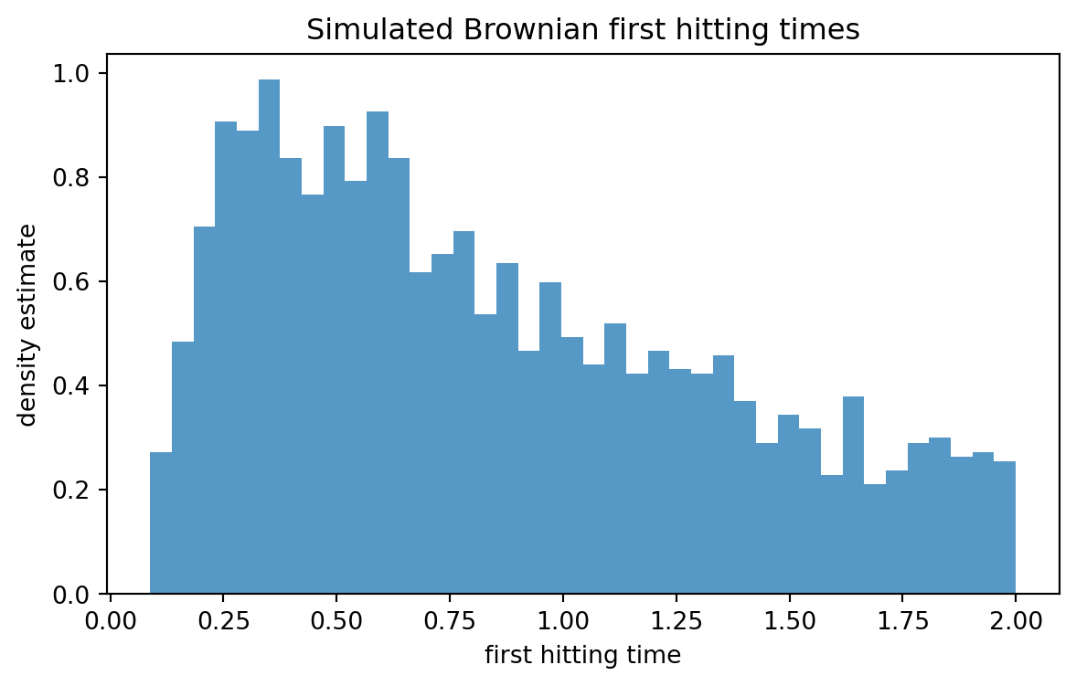
For Brownian motion, a common example is the first hitting time of a level $a$:
$$
\tau_a=\inf\{t\ge 0: W_t=a\}.
$$
If $a>0$, then $\tau_a$ is the first time Brownian motion reaches the upper level $a$.
The reflection principle gives formulas for maxima of Brownian motion. For example,
$$
\mathbb P\left(\max_{0\le s\le T} W_s\ge a\right)
=
2\mathbb P(W_T\ge a),
\qquad a>0.
$$
This formula is important for barrier options, where payoff depends on whether a price process crosses a boundary.
```{python}
#| label: py-ch10-hitting-time-simulation
#| fig-cap: "Simulated first hitting times for Brownian motion crossing level 1."
import numpy as np
import matplotlib.pyplot as plt

rng = np.random.default_rng(7339)
T = 2.0
n = 1000
dt = T / n
m_paths = 5000
level = 1.0

hit_times = []
for _ in range(m_paths):
    dW = rng.normal(0.0, np.sqrt(dt), size=n)
    W = np.cumsum(dW)
    hit_indices = np.where(W >= level)[0]
    if len(hit_indices) > 0:
        hit_times.append((hit_indices[0] + 1) * dt)

hit_times = np.array(hit_times)
print("Fraction of paths hitting level 1 by time T:", round(len(hit_times) / m_paths, 4))

plt.figure(figsize=(7, 4))
plt.hist(hit_times, bins=40, density=True, alpha=0.75)
plt.xlabel("first hitting time")
plt.ylabel("density estimate")
plt.title("Simulated Brownian first hitting times")
plt.show()
```
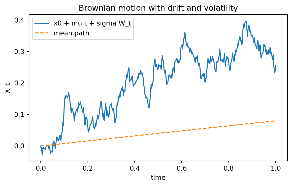
## 10.12 Brownian Motion with Drift and Volatility
A standard Brownian motion has zero mean and variance $t$. In applications, we often use a process with drift and volatility:
$$
X_t=x_0+\mu t+\sigma W_t.
$$
Then
$$
X_t\sim N(x_0+\mu t,\sigma^2t).
$$
The parameter $\mu$ controls the deterministic trend, while $\sigma$ controls the magnitude of random fluctuations.
In finance, a basic continuous-time model for a log price is
$$
\log S_t=\log S_0+\left(\mu-\frac12\sigma^2\right)t+\sigma W_t.
$$
Equivalently,
$$
S_t=S_0\exp\left(\left(\mu-\frac12\sigma^2\right)t+\sigma W_t\right).
$$
This is geometric Brownian motion, which will be developed carefully in Chapter 14. The correction term $-\frac12\sigma^2$ is not arbitrary; it comes from Itô's formula.
```{python}
#| label: py-ch10-brownian-with-drift-volatility
#| fig-cap: "Brownian motion with drift and volatility."
import numpy as np
import matplotlib.pyplot as plt

rng = np.random.default_rng(2026)
T = 1.0
n = 500
dt = T / n
time = np.linspace(0, T, n + 1)

mu = 0.08
sigma = 0.25
x0 = 0.0

dW = rng.normal(0.0, np.sqrt(dt), size=n)
W = np.concatenate([[0.0], np.cumsum(dW)])
X = x0 + mu * time + sigma * W

plt.figure(figsize=(7, 4))
plt.plot(time, X, label="x0 + mu t + sigma W_t")
plt.plot(time, x0 + mu * time, linestyle="--", label="mean path")
plt.xlabel("time")
plt.ylabel("X_t")
plt.title("Brownian motion with drift and volatility")
plt.legend()
plt.show()
```
## 10.13 Simulation Method
To simulate Brownian motion on a grid
$$
0=t_0<t_1<\cdots<t_n=T,
$$
use independent increments
$$
W_{t_{k+1}}-W_{t_k}\sim N(0,t_{k+1}-t_k).
$$
For an equally spaced grid with $\Delta t=T/n$,
$$
\Delta W_k=\sqrt{\Delta t}\,Z_k,
\qquad
Z_k\sim N(0,1).
$$
Then
$$
W_{t_k}=\sum_{j=0}^{k-1}\Delta W_j.
$$
This simulation is exact on the grid points. It is not an approximation to the distribution at those grid points. The approximation is only in how we visualize the continuous path between grid points.
```{python}
#| label: py-ch10-vectorized-simulation
# Vectorized simulation of many Brownian paths.
import numpy as np

rng = np.random.default_rng(9001)
T = 1.0
n = 252
m_paths = 10000
dt = T / n

dW = rng.normal(0.0, np.sqrt(dt), size=(m_paths, n))
W = np.column_stack([np.zeros(m_paths), np.cumsum(dW, axis=1)])
terminal = W[:, -1]

print("Empirical mean of W_T:", round(terminal.mean(), 4))
print("Empirical variance of W_T:", round(terminal.var(ddof=1), 4))
print("Theoretical mean:", 0.0)
print("Theoretical variance:", T)
```
## 10.14 Brownian Motion Is Not Ordinary Differentiable
A differentiable function has increments approximately proportional to $\Delta t$:
$$
f(t+\Delta t)-f(t)\approx f'(t)\Delta t.
$$
Brownian increments have size approximately $\sqrt{\Delta t}$, not $\Delta t$. Indeed,
$$
W_{t+\Delta t}-W_t\sim N(0,\Delta t),
$$
so a typical absolute increment is of order $\sqrt{\Delta t}$.
The difference quotient therefore has size approximately
$$
\frac{\sqrt{\Delta t}}{\Delta t}=\frac{1}{\sqrt{\Delta t}},
$$
which becomes large as $\Delta t\to 0$. This explains why Brownian motion cannot be handled by ordinary differential calculus.
This issue leads directly to stochastic differential notation:
$$
dX_t=\mu(t,X_t)dt+\sigma(t,X_t)dW_t.
$$
The term $dW_t$ is not an ordinary differential. It is interpreted through stochastic integration, which is the topic of Chapter 11.
## 10.15 Financial Meaning: Random Shock, Not Price
A common modeling mistake is to write
$$
S_t=S_0+\sigma W_t
$$
for a stock price. This can become negative. A better first model is to use Brownian motion as the driver of log price:
$$
dS_t=\mu S_tdt+\sigma S_tdW_t.
$$
This stochastic differential equation has a positive solution. The model says that relative changes, not absolute changes, are driven by Brownian shocks.
Brownian motion is useful because it provides:
- a tractable model of continuous random fluctuations;
- Gaussian transition distributions;
- independent increments;
- martingale structure under suitable measures;
- quadratic variation, which makes Itô calculus possible.
It is also limited because real financial markets may have:
- jumps;
- volatility clustering;
- heavy tails;
- transaction costs;
- market microstructure noise;
- changing regimes;
- feedback effects and strategic behavior.
Thus Brownian motion is not the truth of financial markets. It is a mathematically clean baseline model.
## 10.16 AI-Assisted Learning Components
::: {.ai-box}
### AI Activity 10.1: Explain the scaling
Ask an AI tool:
> Explain why the scaling $S_{\lfloor nt\rfloor}/\sqrt n$ is natural when a random walk converges to Brownian motion. Use variance as the main argument and avoid measure-theoretic language.
Then check whether the explanation includes these three points:
1. independent increments make variances add;
2. $nt$ steps have variance approximately $nt$;
3. dividing by $\sqrt n$ produces variance approximately $t$.
:::
::: {.ai-box}
### AI Activity 10.2: Audit a Brownian simulation
Give an AI tool the following pseudocode:
```text
for k in 1,...,n:
    dW[k] = normal(mean = 0, standard_deviation = dt)
    W[k] = W[k-1] + dW[k]
```
Ask it to find the mathematical error. The correct standard deviation should be $\sqrt{dt}$, not $dt$.
:::
::: {.ai-box}
### AI Activity 10.3: Model critique
Ask an AI tool:
> What financial phenomena are not well captured by Brownian motion with constant volatility?
A good answer should mention jumps, heavy tails, volatility clustering, stochastic volatility, regime changes, and market frictions.
:::
## 10.17 Common Mistakes
1. **Confusing levels and increments.** The levels $W_s$ and $W_t$ are correlated, but nonoverlapping increments are independent.
2. **Using $dt$ instead of $\sqrt{dt}$ in simulation.** Brownian increments on a time step of length $dt$ have standard deviation $\sqrt{dt}$.
3. **Thinking Brownian paths are smooth because they are continuous.** Brownian motion is continuous but almost surely nowhere differentiable.
4. **Treating Brownian motion as a stock price.** Brownian motion can be negative. It usually drives log prices or stochastic state variables.
5. **Applying the square-root-of-time rule blindly.** The rule requires strong assumptions that may fail in real data.
6. **Forgetting quadratic variation.** The identity $(dW_t)^2=dt$ is the key reason Itô calculus differs from ordinary calculus.
## 10.18 Chapter Summary
Brownian motion is the central continuous-time noise process in mathematical finance. It arises as the scaling limit of random walks and is characterized by continuous paths, independent Gaussian increments, and variance growing linearly in time.
The key formulas are:
$$
W_t-W_s\sim N(0,t-s),
$$
$$
\operatorname{Cov}(W_s,W_t)=\min(s,t),
$$
$$
\mathbb E[W_t\mid\mathcal F_s]=W_s,
$$
and
$$
\sum_k (W_{t_{k+1}}-W_{t_k})^2\to T.
$$
The last formula is the quadratic variation of Brownian motion. It is the mathematical fact behind the symbolic rule
$$
(dW_t)^2=dt.
$$
This chapter prepares the ground for stochastic integration, Itô's formula, stochastic differential equations, geometric Brownian motion, and the Black--Scholes model.
## 10.19 Exercises
### Conceptual Exercises
1. Explain why Brownian motion is a reasonable first model for cumulative random shocks, but not for a stock price itself.
2. What is the difference between independent increments and independent values? Use $W_1$ and $W_2$ as an example.
3. Explain why $W_t\sim N(0,t)$ implies that uncertainty grows like $\sqrt t$ rather than like $t$.
4. In your own words, explain why Brownian motion is continuous but not differentiable.
5. What does the natural filtration $\mathcal F_t=\sigma(W_s:0\le s\le t)$ represent in a financial model?
### Computational Exercises
6. Compute $\mathbb P(W_2>1)$ for standard Brownian motion.
7. Compute $\operatorname{Cov}(W_{0.5},W_3)$ and $\operatorname{Corr}(W_{0.5},W_3)$.
8. Let $X_t=2+0.04t+0.3W_t$. Find the mean and variance of $X_5$.
9. Suppose daily volatility is $1.5\%$. Use the square-root-of-time rule to estimate 20-day volatility and annualized volatility using 252 trading days.
10. Let $0<s<t$. Prove directly that $\mathbb E[W_t-W_s\mid\mathcal F_s]=0$.
### Proof Exercises
11. Prove that $\operatorname{Cov}(W_s,W_t)=\min(s,t)$.
12. Prove that $W_t^2-t$ is a martingale.
13. Prove that $\exp(\theta W_t-\frac12\theta^2t)$ is a martingale for fixed $\theta$.
14. For an equally spaced partition of $[0,T]$, compute the expectation of the quadratic variation sum.
15. Compute the variance of the quadratic variation sum and show that it converges to $0$ as the mesh size goes to $0$.
### Python Exercises
16. Simulate $10{,}000$ Brownian paths on $[0,1]$ and verify empirically that $W_1$ has mean approximately $0$ and variance approximately $1$.
17. Simulate Brownian motion with drift $X_t=x_0+\mu t+\sigma W_t$. Compare the empirical mean of $X_T$ with $x_0+\mu T$.
18. Estimate the probability $\mathbb P(\max_{0\le t\le 1}W_t\ge 1)$ by simulation and compare it with the reflection-principle formula.
19. Simulate one fine Brownian path and compute ordinary variation and quadratic variation along increasingly fine partitions.
20. Simulate geometric Brownian motion using
$$
S_t=S_0\exp\left(\left(\mu-\frac12\sigma^2\right)t+\sigma W_t\right).
$$
Check that simulated prices remain positive.
### AI-Assisted Exercises
21. Ask an AI tool to explain the difference between Brownian motion and white noise. Then rewrite the explanation in your own words.
22. Ask an AI tool to generate Brownian simulation code. Check whether it uses $\sqrt{dt}$ correctly.
23. Ask an AI tool why Brownian motion has quadratic variation $T$ on $[0,T]$. Identify whether the explanation uses expectation only or also discusses convergence.
24. Ask an AI tool to critique the use of Brownian motion in stock-price modeling. Classify each critique as mathematical, statistical, or market-structure related.
25. Ask an AI tool to produce three examples of financial derivatives whose payoff depends on a hitting time or maximum. Verify the examples mathematically.