---
title: "Chapter 28. Value at Risk and Expected Shortfall"
---
::: {.chapter-objectives}
## Learning Goals
By the end of this chapter, students should be able to:
- define loss variables and explain why risk measurement is usually stated in terms of losses rather than gains;
- compute quantiles, Value at Risk, and Expected Shortfall for discrete, empirical, and continuous loss distributions;
- distinguish sign conventions for returns, portfolio values, and losses;
- derive closed-form VaR and ES formulas under a normal loss model;
- explain why VaR may fail subadditivity and why this matters for diversification;
- state the axioms of coherent risk measures and identify which axioms VaR and ES satisfy;
- estimate VaR and ES using historical simulation, parametric models, and Monte Carlo simulation;
- backtest VaR using exception counts;
- use Python and AI tools to audit risk-measure calculations, code, assumptions, and interpretation.
:::
::: {.hero-box}
A risk measure compresses a loss distribution into a single number. The compression is useful but dangerous: a single number cannot describe the entire tail of a distribution.
Two of the most important tail risk measures are **Value at Risk** and **Expected Shortfall**:
$$
\operatorname{VaR}_{\alpha}(L)
=
\inf\{x\in\mathbb R: \mathbb P(L\le x)\ge \alpha\},
$$
and, for a continuous loss distribution,
$$
\operatorname{ES}_{\alpha}(L)
=
\mathbb E[L\mid L\ge \operatorname{VaR}_{\alpha}(L)].
$$
VaR answers: *How large is a loss threshold that is exceeded only with probability about $1-\alpha$?* ES answers: *If we are in that tail, what is the average loss?*
:::
## 28.1 From Portfolio Value to Loss
Let $V_0$ be the current value of a portfolio and $V_T$ its value at a future horizon $T$. A common loss convention is
$$
L=V_0-V_T.
$$
A positive $L$ means the portfolio lost value. If $R=(V_T-V_0)/V_0$ is the simple portfolio return, then
$$
L=-V_0R.
$$
Thus a large positive loss corresponds to a large negative return. This sign convention is one of the most common sources of mistakes in risk measurement.
::: {.definition}
## Loss variable
A **loss variable** is a real-valued random variable $L$ whose larger values represent worse outcomes. The distribution of $L$ is called the **loss distribution**.
:::
For a one-day equity portfolio, $L$ may represent dollar loss over one trading day. For a credit portfolio, $L$ may represent total default loss over one year. For a derivatives book, $L$ may represent the negative mark-to-market change over a specified horizon.
Risk measures are functions
$$
\rho:L\mapsto \rho(L)
$$
that assign a number to a loss variable. In practice, $\rho(L)$ is often interpreted as capital, margin, or a risk limit.
::: {.remark}
## Same mathematics, different units
If $L$ is measured in dollars, then VaR and ES are measured in dollars. If $L$ is measured as a percentage loss, then VaR and ES are percentages. The formulas are the same, but the interpretation changes.
:::
## 28.2 Quantiles and Distribution Functions
Let $F_L$ be the cumulative distribution function of $L$:
$$
F_L(x)=\mathbb P(L\le x).
$$
For $\alpha\in(0,1)$, the lower $\alpha$-quantile is
$$
q_\alpha(L)=\inf\{x\in\mathbb R:F_L(x)\ge \alpha\}.
$$
This definition works for both continuous and discrete distributions. If $F_L$ is continuous and strictly increasing, then $q_\alpha(L)$ is the unique solution of
$$
F_L(q_\alpha)=\alpha.
$$
If $F_L$ has jumps, there may be no $x$ with $F_L(x)=\alpha$. The infimum definition is used to avoid ambiguity.
::: {.definition}
## Value at Risk
For a loss variable $L$ and confidence level $\alpha\in(0,1)$, the **Value at Risk** at level $\alpha$ is
$$
\operatorname{VaR}_\alpha(L)=q_\alpha(L)
=\inf\{x\in\mathbb R:F_L(x)\ge \alpha\}.
$$
:::
For example, if $\operatorname{VaR}_{0.99}(L)=2{,}000{,}000$, then the interpretation is:
> With the model and horizon being used, losses exceed $2{,}000{,}000$ with probability at most about $1\%$.
This does **not** say that the worst possible loss is $2{,}000{,}000$. It says that $2{,}000{,}000$ is a high quantile of the loss distribution.
## 28.3 Discrete Example
Suppose a loss variable has distribution
$$
\mathbb P(L=0)=0.95,
\qquad
\mathbb P(L=100)=0.04,
\qquad
\mathbb P(L=1000)=0.01.
$$
Then the cumulative distribution is
$$
F_L(x)=
\begin{cases}
0, & x<0,\\
0.95, & 0\le x<100,\\
0.99, & 100\le x<1000,\\
1, & x\ge 1000.
\end{cases}
$$
Therefore,
$$
\operatorname{VaR}_{0.95}(L)=0,
\qquad
\operatorname{VaR}_{0.99}(L)=100,
\qquad
\operatorname{VaR}_{0.995}(L)=1000.
$$
This example shows that VaR can be insensitive to the size of losses beyond the quantile. At the $99\%$ level, VaR is $100$, even though a loss of $1000$ is possible.
::: {.remark}
## VaR is a threshold, not a tail average
VaR describes a point on the loss distribution. It does not describe how severe losses are after the threshold is crossed. This motivates Expected Shortfall.
:::
## 28.4 Expected Shortfall
For continuous loss distributions, Expected Shortfall is the average loss conditional on being in the tail:
$$
\operatorname{ES}_\alpha(L)
=
\mathbb E[L\mid L\ge \operatorname{VaR}_\alpha(L)].
$$
A more robust definition, valid more generally, is the quantile-average formula
$$
\operatorname{ES}_\alpha(L)
=
\frac{1}{1-\alpha}\int_\alpha^1 \operatorname{VaR}_u(L)\,du.
$$
For continuous distributions, these definitions agree under standard integrability assumptions.
::: {.definition}
## Expected Shortfall
Let $L$ be an integrable loss variable and $\alpha\in(0,1)$. The **Expected Shortfall** at level $\alpha$ is
$$
\operatorname{ES}_\alpha(L)
=
\frac{1}{1-\alpha}\int_\alpha^1 \operatorname{VaR}_u(L)\,du.
$$
:::
Expected Shortfall is also called **Conditional Value at Risk**, **CVaR**, or **Average Value at Risk**. In this book we use the name Expected Shortfall because it emphasizes the tail-average interpretation.
For a continuous distribution,
$$
\operatorname{ES}_\alpha(L)\ge \operatorname{VaR}_\alpha(L),
$$
because ES averages losses in the upper tail, while VaR is the lower endpoint of that tail.
## 28.5 Interactive Demo: Normal Loss VaR and ES
The following demo uses a normal loss model
$$
L\sim N(\mu,\sigma^2).
$$
For this model,
$$
\operatorname{VaR}_\alpha(L)=\mu+\sigma z_\alpha,
$$
where $z_\alpha=\Phi^{-1}(\alpha)$, and
$$
\operatorname{ES}_\alpha(L)=\mu+\sigma\frac{\phi(z_\alpha)}{1-\alpha}.
$$
::: {.interactive-card}
### Normal loss distribution: VaR versus ES
<div class="mf-control-row">
<label for="ch28-alpha">Confidence level $\alpha$</label>
<input id="ch28-alpha" type="range" min="0.900" max="0.999" step="0.001" value="0.975">
<span id="ch28-alpha-val" class="mf-badge">0.975</span>
</div>
<div class="mf-control-row">
<label for="ch28-sigma">Loss volatility $\sigma$</label>
<input id="ch28-sigma" type="range" min="0.5" max="3.0" step="0.1" value="1.0">
<span id="ch28-sigma-val" class="mf-badge">1.0</span>
</div>
<div id="ch28-normal-risk-demo" class="plotly-demo"></div>
<div id="ch28-normal-risk-output" class="mf-output"></div>
:::
<script>
mfPlotlyReady(function() {
var alphaSlider = document.getElementById("ch28-alpha");
var sigmaSlider = document.getElementById("ch28-sigma");
var alphaVal = document.getElementById("ch28-alpha-val");
var sigmaVal = document.getElementById("ch28-sigma-val");
var out = document.getElementById("ch28-normal-risk-output");
var plotId = "ch28-normal-risk-demo";
function erf(x) {
var sign = x >= 0 ? 1 : -1;
x = Math.abs(x);
var a1 = 0.254829592, a2 = -0.284496736, a3 = 1.421413741;
var a4 = -1.453152027, a5 = 1.061405429, p = 0.3275911;
var t = 1 / (1 + p * x);
var y = 1 - (((((a5 * t + a4) * t) + a3) * t + a2) * t + a1) * t * Math.exp(-x * x);
return sign * y;
}
function Phi(x) { return 0.5 * (1 + erf(x / Math.sqrt(2))); }
function phi(x) { return Math.exp(-0.5 * x * x) / Math.sqrt(2 * Math.PI); }
function normInv(p) {
// Peter J. Acklam's rational approximation.
var a = [-39.6968302866538, 220.946098424521, -275.928510446969, 138.357751867269, -30.6647980661472, 2.50662827745924];
var b = [-54.4760987982241, 161.585836858041, -155.698979859887, 66.8013118877197, -13.2806815528857];
var c = [-0.00778489400243029, -0.322396458041136, -2.40075827716184, -2.54973253934373, 4.37466414146497, 2.93816398269878];
var d = [0.00778469570904146, 0.32246712907004, 2.445134137143, 3.75440866190742];
var plow = 0.02425, phigh = 1 - plow;
var q, r;
if (p < plow) {
q = Math.sqrt(-2 * Math.log(p));
return (((((c[0] * q + c[1]) * q + c[2]) * q + c[3]) * q + c[4]) * q + c[5]) /
((((d[0] * q + d[1]) * q + d[2]) * q + d[3]) * q + 1);
}
if (p <= phigh) {
q = p - 0.5;
r = q * q;
return (((((a[0] * r + a[1]) * r + a[2]) * r + a[3]) * r + a[4]) * r + a[5]) * q /
(((((b[0] * r + b[1]) * r + b[2]) * r + b[3]) * r + b[4]) * r + 1);
}
q = Math.sqrt(-2 * Math.log(1 - p));
return -(((((c[0] * q + c[1]) * q + c[2]) * q + c[3]) * q + c[4]) * q + c[5]) /
((((d[0] * q + d[1]) * q + d[2]) * q + d[3]) * q + 1);
}
function draw() {
var alpha = parseFloat(alphaSlider.value);
var sigma = parseFloat(sigmaSlider.value);
var mu = 0.0;
alphaVal.textContent = alpha.toFixed(3);
sigmaVal.textContent = sigma.toFixed(1);
var z = normInv(alpha);
var varValue = mu + sigma * z;
var esValue = mu + sigma * phi(z) / (1 - alpha);
var xs = [], ys = [], tailX = [], tailY = [];
var lo = mu - 4 * sigma, hi = mu + 5 * sigma;
for (var i = 0; i <= 350; i++) {
var x = lo + (hi - lo) * i / 350;
var y = phi((x - mu) / sigma) / sigma;
xs.push(x); ys.push(y);
if (x >= varValue) { tailX.push(x); tailY.push(y); }
}
var traces = [
{x: xs, y: ys, mode: "lines", name: "loss density"},
{x: tailX.concat([hi, varValue]), y: tailY.concat([0, 0]), fill: "toself", mode: "lines", name: "tail beyond VaR", line: {width: 0}},
{x: [varValue, varValue], y: [0, phi(z) / sigma], mode: "lines", name: "VaR"},
{x: [esValue], y: [0], mode: "markers+text", text: ["ES"], textposition: "top center", name: "ES", marker: {size: 11}}
];
var layout = {
title: "Normal loss: VaR is a quantile, ES is a tail mean",
xaxis: {title: "loss"},
yaxis: {title: "density"},
margin: {l: 60, r: 25, t: 55, b: 55},
legend: {orientation: "h"}
};
Plotly.newPlot(plotId, traces, layout, {responsive: true});
out.innerHTML = "VaR = " + varValue.toFixed(3) + ", ES = " + esValue.toFixed(3) + ". The gap grows as the confidence level moves deeper into the tail.";
}
alphaSlider.addEventListener("input", draw);
sigmaSlider.addEventListener("input", draw);
draw();
});
</script>
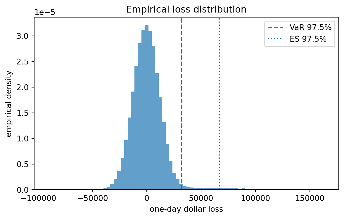
## 28.6 Python Example: Empirical VaR and ES
The empirical method treats observed or simulated losses as samples from the loss distribution. If the sample losses are
$$
L_1,\ldots,L_n,
$$
then the empirical VaR is a sample quantile and the empirical ES is the average of losses beyond that quantile.
```{python}
#| label: ch28-empirical-var-es
#| echo: true
#| warning: false
#| message: false
import numpy as np
import pandas as pd

rng = np.random.default_rng(7243)
n = 100_000
alpha = 0.975

# Simulated daily portfolio returns: a mixture model with rare stressful days.
normal_days = rng.normal(loc=0.0005, scale=0.012, size=n)
stress_days = rng.normal(loc=-0.055, scale=0.035, size=n)
stress_indicator = rng.uniform(size=n) < 0.03
returns = np.where(stress_indicator, stress_days, normal_days)

initial_value = 1_000_000
losses = -initial_value * returns

var_emp = np.quantile(losses, alpha, method="higher")
es_emp = losses[losses >= var_emp].mean()

pd.DataFrame({
    "risk measure": [f"VaR {alpha:.1%}", f"ES {alpha:.1%}"],
    "dollar value": [var_emp, es_emp]
})
```
The empirical ES is larger than the empirical VaR because it averages losses after the VaR threshold is crossed. In a heavy-tailed or mixture distribution, this gap may be large.
```{python}
#| label: ch28-loss-histogram
#| echo: true
#| warning: false
#| message: false
import matplotlib.pyplot as plt

plt.figure(figsize=(7, 4))
plt.hist(losses, bins=80, density=True, alpha=0.7)
plt.axvline(var_emp, linestyle="--", label=f"VaR {alpha:.1%}")
plt.axvline(es_emp, linestyle=":", label=f"ES {alpha:.1%}")
plt.xlabel("one-day dollar loss")
plt.ylabel("empirical density")
plt.title("Empirical loss distribution")
plt.legend()
plt.show()
```
## 28.7 Normal Model Formulas
Suppose
$$
L\sim N(\mu,\sigma^2).
$$
Let $Z=(L-\mu)/\sigma\sim N(0,1)$, and let $z_\alpha=\Phi^{-1}(\alpha)$. Then
$$
\operatorname{VaR}_\alpha(L)
=\mu+\sigma z_\alpha.
$$
For Expected Shortfall, first compute
$$
\mathbb E[Z\mid Z\ge z_\alpha]
=
\frac{\phi(z_\alpha)}{1-\alpha}.
$$
Therefore,
$$
\operatorname{ES}_\alpha(L)
=\mu+\sigma\frac{\phi(z_\alpha)}{1-\alpha}.
$$
::: {.proof}
## Derivation of the normal ES formula
For $Z\sim N(0,1)$,
$$
\mathbb E[Z\mathbf 1_{\{Z\ge z\}}]
=\int_z^\infty x\phi(x)\,dx.
$$
Since $\phi'(x)=-x\phi(x)$,
$$
\int_z^\infty x\phi(x)\,dx
=\int_z^\infty -\phi'(x)\,dx
=\phi(z).
$$
Thus
$$
\mathbb E[Z\mid Z\ge z]
=\frac{\mathbb E[Z\mathbf 1_{\{Z\ge z\}}]}{\mathbb P(Z\ge z)}
=\frac{\phi(z)}{1-\Phi(z)}.
$$
Taking $z=z_\alpha$ gives the result.
:::
```{python}
#| label: ch28-normal-formulas
#| echo: true
#| warning: false
#| message: false
from scipy.stats import norm

mu = 10_000
sigma = 50_000
alpha_grid = np.array([0.95, 0.975, 0.99])

z = norm.ppf(alpha_grid)
var_normal = mu + sigma * z
es_normal = mu + sigma * norm.pdf(z) / (1 - alpha_grid)

pd.DataFrame({
    "alpha": alpha_grid,
    "z_alpha": z,
    "VaR": var_normal,
    "ES": es_normal,
    "ES - VaR": es_normal - var_normal
})
```
## 28.8 Heavy Tails and Model Risk
The normal model is analytically convenient but often underestimates tail risk. A Student-$t$ model with low degrees of freedom has heavier tails.
Let $X$ be a standardized Student-$t$ random variable and define a loss model
$$
L=\mu+\sigma X.
$$
If $X$ is scaled to have variance one, it may match the mean and variance of a normal model while producing much larger VaR and ES at high confidence levels.
```{python}
#| label: ch28-heavy-tail-comparison
#| echo: true
#| warning: false
#| message: false
from scipy.stats import t

rng = np.random.default_rng(5110)
n = 300_000
alpha = 0.99
mu = 0.0
sigma = 1.0
nu = 4

normal_losses = rng.normal(mu, sigma, size=n)
# Scale t_nu to have variance 1: Var(t_nu)=nu/(nu-2), for nu>2.
t_losses = rng.standard_t(df=nu, size=n) * np.sqrt((nu - 2) / nu)

def empirical_var_es(x, alpha):
    var = np.quantile(x, alpha, method="higher")
    es = x[x >= var].mean()
    return var, es

var_n, es_n = empirical_var_es(normal_losses, alpha)
var_t, es_t = empirical_var_es(t_losses, alpha)

pd.DataFrame({
    "model": ["standard normal", f"standardized t(df={nu})"],
    "VaR 99%": [var_n, var_t],
    "ES 99%": [es_n, es_t]
})
```
::: {.remark}
## Matching volatility is not enough
Two models may have the same mean and variance but very different tail risk. VaR and ES depend on the full tail of the loss distribution, not only on volatility.
:::
## 28.9 Coherent Risk Measures
A risk measure $\rho$ maps loss variables to real numbers. A widely used mathematical standard is coherence.
::: {.definition}
## Coherent risk measure
A risk measure $\rho$ is **coherent** if it satisfies the following four properties for loss variables $L,L_1,L_2$, constants $c\in\mathbb R$, and scalars $a\ge0$:
1. **Monotonicity:** if $L_1\le L_2$ almost surely, then
$$
\rho(L_1)\le \rho(L_2).
$$
2. **Translation invariance:**
$$
\rho(L+c)=\rho(L)+c.
$$
3. **Positive homogeneity:**
$$
\rho(aL)=a\rho(L).
$$
4. **Subadditivity:**
$$
\rho(L_1+L_2)\le \rho(L_1)+\rho(L_2).
$$
:::
Subadditivity expresses the mathematical principle that diversification should not increase measured risk. If a risk measure violates subadditivity, then it may penalize diversification.
VaR satisfies monotonicity, translation invariance, and positive homogeneity under standard definitions. However, VaR may fail subadditivity. Expected Shortfall is coherent under standard integrability assumptions.
## 28.10 Interactive Demo: VaR Can Fail Subadditivity
Consider two independent default-type losses:
$$
L_i=
\begin{cases}
100, & \text{with probability }p,\\
0, & \text{with probability }1-p,
\end{cases}
\qquad i=1,2.
$$
If $p<1-\alpha$, then each single position has
$$
\operatorname{VaR}_\alpha(L_i)=0.
$$
But the diversified portfolio $L_1+L_2$ may have positive VaR because the probability that at least one default occurs can exceed $1-\alpha$.
::: {.interactive-card}
### VaR subadditivity stress test
<div class="mf-control-row">
<label for="ch28-default-p">Default probability $p$</label>
<input id="ch28-default-p" type="range" min="0.005" max="0.080" step="0.001" value="0.030">
<span id="ch28-default-p-val" class="mf-badge">0.030</span>
</div>
<div class="mf-control-row">
<label for="ch28-sub-alpha">Confidence level $\alpha$</label>
<input id="ch28-sub-alpha" type="range" min="0.900" max="0.995" step="0.001" value="0.950">
<span id="ch28-sub-alpha-val" class="mf-badge">0.950</span>
</div>
<div id="ch28-subadditivity-demo" class="plotly-demo"></div>
<div id="ch28-subadditivity-output" class="mf-output"></div>
:::
<script>
mfPlotlyReady(function() {
var pSlider = document.getElementById("ch28-default-p");
var alphaSlider = document.getElementById("ch28-sub-alpha");
var pVal = document.getElementById("ch28-default-p-val");
var alphaVal = document.getElementById("ch28-sub-alpha-val");
var out = document.getElementById("ch28-subadditivity-output");
var plotId = "ch28-subadditivity-demo";
function discreteVaR(values, probs, alpha) {
var pairs = values.map(function(v, i) { return {v: v, p: probs[i]}; }).sort(function(a, b) { return a.v - b.v; });
var c = 0;
for (var i = 0; i < pairs.length; i++) {
c += pairs[i].p;
if (c >= alpha - 1e-12) return pairs[i].v;
}
return pairs[pairs.length - 1].v;
}
function discreteES(values, probs, alpha) {
var pairs = values.map(function(v, i) { return {v: v, p: probs[i]}; }).sort(function(a, b) { return a.v - b.v; });
var tailProb = 1 - alpha;
var remaining = tailProb;
var total = 0;
for (var i = pairs.length - 1; i >= 0 && remaining > 1e-12; i--) {
var take = Math.min(remaining, pairs[i].p);
total += take * pairs[i].v;
remaining -= take;
}
return total / tailProb;
}
function draw() {
var p = parseFloat(pSlider.value);
var alpha = parseFloat(alphaSlider.value);
pVal.textContent = p.toFixed(3);
alphaVal.textContent = alpha.toFixed(3);
var varSingle = discreteVaR([0, 100], [1 - p, p], alpha);
var esSingle = discreteES([0, 100], [1 - p, p], alpha);
var values = [0, 100, 200];
var probs = [(1 - p) * (1 - p), 2 * p * (1 - p), p * p];
var varSum = discreteVaR(values, probs, alpha);
var esSum = discreteES(values, probs, alpha);
var traces = [
{x: values.map(String), y: probs, type: "bar", name: "P(L1+L2=x)"},
{x: [String(varSum)], y: [Math.max.apply(null, probs)], mode: "markers+text", text: ["VaR"], textposition: "top center", name: "portfolio VaR", marker: {size: 12}}
];
var layout = {
title: "Distribution of the combined loss L1 + L2",
xaxis: {title: "combined loss"},
yaxis: {title: "probability", tickformat: ".1%"},
margin: {l: 60, r: 25, t: 55, b: 55},
legend: {orientation: "h"}
};
Plotly.newPlot(plotId, traces, layout, {responsive: true});
var lhs = varSum;
var rhs = 2 * varSingle;
var status = lhs <= rhs ? "Subadditivity holds in this setting." : "VaR violates subadditivity in this setting.";
out.innerHTML = "VaR(L1) = " + varSingle.toFixed(0) + ", VaR(L2) = " + varSingle.toFixed(0) + ", VaR(L1+L2) = " + varSum.toFixed(0) + ". " + status + " ES comparison: ES(L1+L2) = " + esSum.toFixed(2) + ", ES(L1)+ES(L2) = " + (2 * esSingle).toFixed(2) + ".";
}
pSlider.addEventListener("input", draw);
alphaSlider.addEventListener("input", draw);
draw();
});
</script>
## 28.11 A Concrete VaR Counterexample
Let $\alpha=0.95$ and suppose
$$
\mathbb P(L_i=100)=0.04,
\qquad
\mathbb P(L_i=0)=0.96,
$$
with $L_1$ and $L_2$ independent. Then
$$
\operatorname{VaR}_{0.95}(L_1)=0,
\qquad
\operatorname{VaR}_{0.95}(L_2)=0.
$$
But
$$
\mathbb P(L_1+L_2=0)=0.96^2=0.9216,
$$
so the $95\%$ quantile of $L_1+L_2$ is $100$:
$$
\operatorname{VaR}_{0.95}(L_1+L_2)=100.
$$
Therefore,
$$
\operatorname{VaR}_{0.95}(L_1+L_2)
=100
>
0+0
=
\operatorname{VaR}_{0.95}(L_1)+\operatorname{VaR}_{0.95}(L_2).
$$
VaR violates subadditivity in this example.
```{python}
#| label: ch28-var-subadditivity-counterexample
#| echo: true
#| warning: false
#| message: false
alpha = 0.95
p = 0.04

# Exact distribution of one default-type loss.
single_values = np.array([0, 100])
single_probs = np.array([1 - p, p])

# Exact distribution of the sum of two independent losses.
sum_values = np.array([0, 100, 200])
sum_probs = np.array([(1 - p)**2, 2 * p * (1 - p), p**2])

def discrete_var(values, probs, alpha):
    order = np.argsort(values)
    values = values[order]
    probs = probs[order]
    cdf = np.cumsum(probs)
    return values[np.searchsorted(cdf, alpha, side="left")]

def discrete_es_quantile_average(values, probs, alpha, grid_size=200_000):
    # Numerical quantile-average ES. This works well for teaching and small examples.
    u_grid = np.linspace(alpha, 1, grid_size, endpoint=False)
    return np.mean([discrete_var(values, probs, u) for u in u_grid])

var_single = discrete_var(single_values, single_probs, alpha)
var_sum = discrete_var(sum_values, sum_probs, alpha)
es_single = discrete_es_quantile_average(single_values, single_probs, alpha)
es_sum = discrete_es_quantile_average(sum_values, sum_probs, alpha)

pd.DataFrame({
    "quantity": ["VaR(L1)", "VaR(L2)", "VaR(L1+L2)", "ES(L1)", "ES(L2)", "ES(L1+L2)"],
    "value": [var_single, var_single, var_sum, es_single, es_single, es_sum]
})
```
## 28.12 Historical, Parametric, and Monte Carlo VaR
There are three common modeling routes.
### Historical simulation
Historical simulation uses past realized losses:
$$
\widehat{\operatorname{VaR}}_\alpha
=
\text{empirical }\alpha\text{-quantile of }L_1,\ldots,L_n.
$$
It is simple and transparent, but it assumes the historical sample is relevant for the future.
### Parametric VaR
Parametric VaR assumes a distributional model. For example, if
$$
L\sim N(\mu,\sigma^2),
$$
then
$$
\widehat{\operatorname{VaR}}_\alpha
=\widehat\mu+\widehat\sigma z_\alpha.
$$
The method is efficient if the distribution is correct, but it can be fragile when tails are misspecified.
### Monte Carlo VaR
Monte Carlo VaR simulates possible future scenarios under a model. If $L^{(1)},\ldots,L^{(M)}$ are simulated losses, then VaR and ES are estimated from the simulated sample.
Monte Carlo methods are flexible and can handle nonlinear portfolios, but they require careful model validation.
```{python}
#| label: ch28-historical-parametric-monte-carlo
#| echo: true
#| warning: false
#| message: false
from scipy.stats import norm

rng = np.random.default_rng(2028)
alpha = 0.99
n_hist = 750
portfolio_value = 1_000_000

# Synthetic historical returns with mild heavy tails.
historical_returns = 0.0003 + 0.012 * rng.standard_t(df=5, size=n_hist) / np.sqrt(5 / 3)
historical_losses = -portfolio_value * historical_returns

# Historical simulation.
var_hist = np.quantile(historical_losses, alpha, method="higher")
es_hist = historical_losses[historical_losses >= var_hist].mean()

# Parametric normal model fitted to historical losses.
mu_hat = historical_losses.mean()
sigma_hat = historical_losses.std(ddof=1)
z = norm.ppf(alpha)
var_param = mu_hat + sigma_hat * z
es_param = mu_hat + sigma_hat * norm.pdf(z) / (1 - alpha)

# Monte Carlo from the fitted normal model.
mc_losses = rng.normal(mu_hat, sigma_hat, size=250_000)
var_mc = np.quantile(mc_losses, alpha, method="higher")
es_mc = mc_losses[mc_losses >= var_mc].mean()

pd.DataFrame({
    "method": ["historical", "parametric normal", "Monte Carlo normal"],
    "VaR 99%": [var_hist, var_param, var_mc],
    "ES 99%": [es_hist, es_param, es_mc]
})
```
## 28.13 Delta-Normal VaR for a Portfolio
Suppose a portfolio has weights $w\in\mathbb R^d$ in risky assets whose one-period return vector is $R$. Let
$$
\mu=\mathbb E[R],
\qquad
\Sigma=\operatorname{Cov}(R).
$$
The portfolio return is
$$
R_p=w^\top R.
$$
If $R$ is modeled as multivariate normal, then
$$
R_p\sim N(w^\top\mu,w^\top\Sigma w).
$$
For portfolio value $V_0$, the loss is
$$
L=-V_0R_p.
$$
Thus
$$
L\sim N(-V_0w^\top\mu,V_0^2w^\top\Sigma w).
$$
Therefore,
$$
\operatorname{VaR}_\alpha(L)
=-V_0w^\top\mu+V_0\sqrt{w^\top\Sigma w}\,z_\alpha,
$$
and
$$
\operatorname{ES}_\alpha(L)
=-V_0w^\top\mu
+V_0\sqrt{w^\top\Sigma w}\frac{\phi(z_\alpha)}{1-\alpha}.
$$
This is called **delta-normal VaR** when the portfolio value is approximated linearly with respect to risk-factor changes.
```{python}
#| label: ch28-delta-normal-var
#| echo: true
#| warning: false
#| message: false
from scipy.stats import norm

V0 = 2_000_000
w = np.array([0.50, 0.30, 0.20])
mu = np.array([0.0004, 0.0002, 0.0003])
vol = np.array([0.015, 0.010, 0.012])
corr = np.array([
    [1.00, 0.35, 0.25],
    [0.35, 1.00, 0.40],
    [0.25, 0.40, 1.00]
])
Sigma = np.outer(vol, vol) * corr

mean_return = w @ mu
vol_return = np.sqrt(w @ Sigma @ w)
alpha = 0.99
z = norm.ppf(alpha)

var_delta_normal = -V0 * mean_return + V0 * vol_return * z
es_delta_normal = -V0 * mean_return + V0 * vol_return * norm.pdf(z) / (1 - alpha)

pd.DataFrame({
    "quantity": ["portfolio mean return", "portfolio volatility", "VaR 99%", "ES 99%"],
    "value": [mean_return, vol_return, var_delta_normal, es_delta_normal]
})
```
## 28.14 Backtesting VaR
Suppose a model produces daily VaR estimates $\widehat v_t$ at level $\alpha$. Let the realized loss on day $t$ be $L_t$. A VaR **exception** occurs when
$$
L_t>\widehat v_t.
$$
If the VaR model is correctly calibrated and exceptions are independent, then the exception indicator
$$
I_t=\mathbf 1_{\{L_t>\widehat v_t\}}
$$
has approximately
$$
I_t\sim \operatorname{Bernoulli}(1-\alpha).
$$
Over $n$ days, the total number of exceptions
$$
N=\sum_{t=1}^n I_t
$$
approximately follows
$$
N\sim \operatorname{Binomial}(n,1-\alpha).
$$
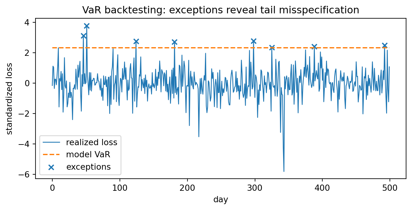
Backtesting compares the observed number and clustering of exceptions to what the model predicts.
```{python}
#| label: ch28-var-backtesting
#| echo: true
#| warning: false
#| message: false
from scipy.stats import binom

alpha = 0.99
n_days = 250
observed_exceptions = np.arange(0, 11)
probabilities = binom.pmf(observed_exceptions, n_days, 1 - alpha)

table = pd.DataFrame({
    "exceptions in 250 days": observed_exceptions,
    "probability under correct 99% VaR": probabilities
})
table
```
```{python}
#| label: ch28-simulated-backtest
#| echo: true
#| warning: false
#| message: false
rng = np.random.default_rng(2029)
n_days = 500
alpha = 0.99

# True losses are heavy-tailed, but the risk model uses a normal VaR estimate.
true_losses = rng.standard_t(df=4, size=n_days) / np.sqrt(4 / 2)
normal_var = norm.ppf(alpha) * np.ones(n_days)
exceptions = true_losses > normal_var

print("Number of exceptions:", exceptions.sum())
print("Expected exceptions under a correct 99% VaR model:", n_days * (1 - alpha))

plt.figure(figsize=(8, 3.5))
plt.plot(true_losses, linewidth=1, label="realized loss")
plt.plot(normal_var, linestyle="--", label="model VaR")
plt.scatter(np.where(exceptions)[0], true_losses[exceptions], marker="x", label="exceptions")
plt.xlabel("day")
plt.ylabel("standardized loss")
plt.title("VaR backtesting: exceptions reveal tail misspecification")
plt.legend()
plt.show()
```
## 28.15 Stress Testing and Scenario Analysis
VaR and ES are model-based summaries. They should be supplemented with stress tests. A stress test asks what happens under specified adverse scenarios, such as:
- equity index falls by $8\%$;
- interest rates shift upward by $100$ basis points;
- credit spreads widen sharply;
- volatility doubles;
- multiple risk factors move together during a liquidity crisis.
Mathematically, a scenario is a vector of risk-factor changes
$$
\Delta X=s.
$$
A portfolio loss under that scenario is
$$
L(s)=V(X_0)-V(X_0+s).
$$
Unlike VaR, a stress test does not require assigning a probability to the scenario. This is valuable when rare events are difficult to estimate statistically.
::: {.remark}
## VaR, ES, and stress testing answer different questions
VaR asks for a high quantile. ES asks for a tail average. Stress testing asks what happens under selected scenarios. A mature risk system uses all three.
:::
## 28.16 AI-Assisted Learning Components
AI tools can be helpful for checking risk-measure calculations, but they should not be trusted blindly. Risk measurement is especially vulnerable to sign errors, tail-direction errors, and unjustified distributional assumptions.
::: {.ai-box}
## AI prompt: Sign-convention audit
Give an AI assistant the following task:
> I define return by $R=(V_T-V_0)/V_0$ and loss by $L=V_0-V_T$. Derive the relationship between $L$ and $R$. Then explain whether the $99\%$ VaR of the return distribution uses a left-tail or right-tail quantile. Give a numerical example.
Check that the response clearly distinguishes the left tail of returns from the right tail of losses.
:::
::: {.ai-box}
## AI prompt: VaR versus ES explanation
Ask an AI assistant:
> Explain why two loss distributions can have the same $99\%$ VaR but very different Expected Shortfall. Give a discrete example with probabilities and losses.
A good response should construct two distributions whose $99\%$ quantiles match but whose losses beyond that quantile are different.
:::
::: {.ai-box}
## AI prompt: Code review for empirical ES
Ask an AI assistant to review the following pseudocode:
```text
var = quantile(losses, alpha)
es = mean(losses[losses <= var])
```
The assistant should identify that the inequality is wrong for a loss variable if ES is meant to average the upper tail. It should use `losses >= var`, with careful handling of ties in discrete samples.
:::
## 28.17 Common Mistakes
1. **Using the wrong tail.** For losses, VaR uses an upper-tail quantile. For returns, large losses correspond to lower-tail returns.
2. **Interpreting VaR as a maximum loss.** Losses can exceed VaR.
3. **Ignoring losses beyond VaR.** VaR does not measure tail severity after the threshold.
4. **Assuming normal tails.** Normal models may underestimate extreme losses.
5. **Forgetting the horizon.** A one-day VaR and a ten-day VaR are not the same object.
6. **Comparing VaR numbers with different confidence levels.** A $95\%$ VaR and a $99\%$ VaR are not directly comparable without context.
7. **Using square-root-of-time scaling blindly.** Scaling rules require assumptions such as independence, stationarity, and finite variance.
8. **Treating backtesting as proof.** Passing a backtest does not prove the model is correct; it only means the observed exceptions were not obviously inconsistent with the model.
## 28.18 Chapter Summary
This chapter introduced risk measures as mathematical functionals of loss distributions. VaR is a quantile:
$$
\operatorname{VaR}_\alpha(L)=\inf\{x:F_L(x)\ge \alpha\}.
$$
Expected Shortfall is a tail average:
$$
\operatorname{ES}_\alpha(L)=\frac{1}{1-\alpha}\int_\alpha^1\operatorname{VaR}_u(L)\,du.
$$
VaR is intuitive and widely used, but it can fail subadditivity and can ignore the severity of losses beyond the quantile. ES is more sensitive to tail severity and is coherent under standard assumptions. Practical risk measurement combines historical simulation, parametric models, Monte Carlo simulation, backtesting, and stress testing.
## 28.19 Exercises
### Conceptual exercises
1. Explain the difference between a return variable and a loss variable. Why does this difference matter for quantiles?
2. Explain why VaR is not a worst-case loss.
3. Explain why Expected Shortfall is usually larger than VaR for continuous loss distributions.
4. Describe a situation in which two portfolios have the same VaR but different ES.
5. Explain why stress testing is still useful even if VaR and ES have already been computed.
### Mathematical exercises
6. Let $L\sim N(\mu,\sigma^2)$. Derive the formulas for $\operatorname{VaR}_\alpha(L)$ and $\operatorname{ES}_\alpha(L)$.
7. Let $L$ have distribution $\mathbb P(L=0)=0.97$ and $\mathbb P(L=100)=0.03$. Compute $\operatorname{VaR}_{0.95}(L)$, $\operatorname{VaR}_{0.99}(L)$, and $\operatorname{ES}_{0.95}(L)$ using the quantile-average definition.
8. Prove translation invariance of VaR:
$$
\operatorname{VaR}_\alpha(L+c)=\operatorname{VaR}_\alpha(L)+c.
$$
9. Prove positive homogeneity of VaR for $a\ge0$:
$$
\operatorname{VaR}_\alpha(aL)=a\operatorname{VaR}_\alpha(L).
$$
10. Construct a discrete example showing that VaR may fail subadditivity.
### Computational exercises
11. Simulate $100{,}000$ losses from a normal distribution and estimate VaR and ES at $95\%$, $97.5\%$, and $99\%$.
12. Repeat Exercise 11 using a standardized Student-$t$ distribution with $4$ degrees of freedom. Compare with the normal model.
13. Write a function that computes empirical VaR and ES from a vector of losses.
14. Simulate two independent default losses and reproduce the VaR subadditivity counterexample.
15. Backtest a rolling historical VaR model on simulated returns with volatility clustering.
### AI-assisted exercises
16. Ask an AI assistant to explain the difference between VaR and ES. Identify one place where the explanation needs more mathematical precision.
17. Ask an AI assistant to derive the normal ES formula. Check whether it correctly uses $\phi'(x)=-x\phi(x)$.
18. Ask an AI assistant to review your empirical VaR and ES code. Verify that it uses the correct tail for losses.
19. Ask an AI assistant to generate a VaR subadditivity counterexample. Check the probabilities and quantiles manually.
20. Ask an AI assistant to compare historical, parametric, and Monte Carlo VaR. Rewrite the response in your own words using precise assumptions.