import numpy as np
import pandas as pd
import matplotlib.pyplot as plt

from math import exp, log, sqrt
from scipy.stats import norm
from scipy.optimize import brentq, minimize37 Python Reference for Mathematical Finance
A Practical Coding Guide for the Computer Labs
38 Python Reference for Mathematical Finance
This page is a practical Python reference for the computer labs in Mathematical Finance. It is not meant to replace a full programming textbook. Instead, it collects the tools, patterns, and numerical ideas that appear repeatedly in the labs.
The book repository is:
https://github.com/wanghemath/Book-MathFinance
The labs are designed to open directly in Google Colab. A typical lab link has the form
https://colab.research.google.com/github/wanghemath/Book-MathFinance/blob/main/labs/lab-01-foundations-returns-no-arbitrage.ipynb38.1 Main Python packages
Most labs use only standard scientific Python packages available in Google Colab:
The main packages are:
| Package | Main use in this book |
|---|---|
numpy |
arrays, vectorized simulation, linear algebra, random numbers |
pandas |
return tables, time series, data summaries |
matplotlib |
plots for prices, payoffs, distributions, yield curves, risk forecasts |
scipy.stats |
normal distribution, random variables, probability functions |
scipy.optimize |
root finding, implied volatility, calibration, portfolio optimization |
38.2 Colab workflow
Each lab is intended to be self-contained. A good student workflow is:
- Open the notebook in Google Colab.
- Run cells from top to bottom.
- Read the mathematical background before running the code.
- Change parameters and rerun important cells.
- Complete the checkpoint questions and exercises.
- Save a personal copy in Google Drive or download the completed notebook.
In Colab, if a package is missing, install it with:
# Example only. Most labs do not require additional installation.
# !pip install yfinance
For the core labs, external data downloads are avoided whenever possible. Synthetic data are used so that the notebooks remain stable and reproducible.
39 NumPy Basics
39.1 Arrays
A NumPy array stores numerical data efficiently.
prices = np.array([100, 101.5, 99.8, 103.2, 104.0])
prices
array([100. , 101.5, 99.8, 103.2, 104. ])Basic operations are vectorized:
prices + 1array([101. , 102.5, 100.8, 104.2, 105. ])prices / prices[0]array([1. , 1.015, 0.998, 1.032, 1.04 ])39.2 Useful array constructors
np.zeros(5)array([0., 0., 0., 0., 0.])np.ones(5)array([1., 1., 1., 1., 1.])np.linspace(0, 1, 6)array([0. , 0.2, 0.4, 0.6, 0.8, 1. ])np.arange(0, 10, 2)array([0, 2, 4, 6, 8])39.3 Vectorization
Vectorization means applying operations to entire arrays instead of writing loops. For example, simple returns are
\[ R_t = \frac{S_t-S_{t-1}}{S_{t-1}}. \]
simple_returns = prices[1:] / prices[:-1] - 1
simple_returns
array([ 0.015 , -0.01674877, 0.03406814, 0.00775194])Log returns are
\[ r_t = \log\left(\frac{S_t}{S_{t-1}}\right). \]
log_returns = np.diff(np.log(prices))
log_returns
array([ 0.01488861, -0.01689062, 0.03350067, 0.00772205])39.4 Summary statistics
returns = np.array([0.01, -0.02, 0.015, 0.005, -0.01])

mean_return = returns.mean()
volatility = returns.std(ddof=1)

mean_return, volatility
(-3.4694469519536144e-19, 0.01457737973711325)The argument ddof=1 gives the sample standard deviation.
40 Random Numbers and Reproducibility
For simulations, use NumPy’s random number generator:
rng = np.random.default_rng(2026)Using a seed makes the simulation reproducible.
rng.normal(loc=0, scale=1, size=5)array([-0.79312248, 0.24057128, -1.89632635, 1.39577171, 0.63829474])Common random draws:
normal_draws = rng.normal(0, 1, size=10)
uniform_draws = rng.uniform(0, 1, size=10)
choice_draws = rng.choice(["up", "down"], size=10, p=[0.55, 0.45])

normal_draws[:3], uniform_draws[:3], choice_draws[:3]
(array([-0.29204749, -0.31194933, 0.30383537]),
array([0.82589526, 0.44838055, 0.33881245]),
array(['up', 'up', 'down'], dtype='<U4'))41 pandas Basics
pandas is useful for organizing financial data in tables.
df = pd.DataFrame({
    "date": pd.date_range("2026-01-01", periods=5, freq="D"),
    "price": [100, 101.5, 99.8, 103.2, 104.0]
})

df| date | price | |
|---|---|---|
| 0 | 2026-01-01 | 100.0 |
| 1 | 2026-01-02 | 101.5 |
| 2 | 2026-01-03 | 99.8 |
| 3 | 2026-01-04 | 103.2 |
| 4 | 2026-01-05 | 104.0 |
Set the date column as the index:
df = df.set_index("date")
df| price | |
|---|---|
| date | |
| 2026-01-01 | 100.0 |
| 2026-01-02 | 101.5 |
| 2026-01-03 | 99.8 |
| 2026-01-04 | 103.2 |
| 2026-01-05 | 104.0 |
Compute returns:
df["simple_return"] = df["price"].pct_change()
df["log_return"] = np.log(df["price"]).diff()
df| price | simple_return | log_return | |
|---|---|---|---|
| date | |||
| 2026-01-01 | 100.0 | NaN | NaN |
| 2026-01-02 | 101.5 | 0.015000 | 0.014889 |
| 2026-01-03 | 99.8 | -0.016749 | -0.016891 |
| 2026-01-04 | 103.2 | 0.034068 | 0.033501 |
| 2026-01-05 | 104.0 | 0.007752 | 0.007722 |
Drop missing values:
df_returns = df.dropna()
df_returns| price | simple_return | log_return | |
|---|---|---|---|
| date | |||
| 2026-01-02 | 101.5 | 0.015000 | 0.014889 |
| 2026-01-03 | 99.8 | -0.016749 | -0.016891 |
| 2026-01-04 | 103.2 | 0.034068 | 0.033501 |
| 2026-01-05 | 104.0 | 0.007752 | 0.007722 |
42 Plotting with matplotlib
42.1 Line plots
plt.figure(figsize=(7, 4))
plt.plot(df.index, df["price"], marker="o")
plt.xlabel("Date")
plt.ylabel("Price")
plt.title("Synthetic Price Series")
plt.grid(True, alpha=0.3)
plt.show()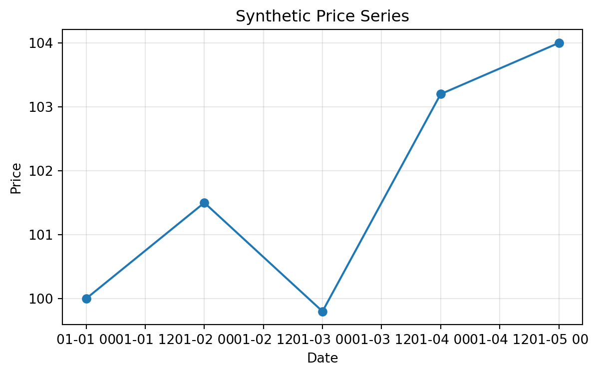
42.2 Histograms
rng = np.random.default_rng(7)
sample_returns = rng.normal(0.0005, 0.02, size=1000)

plt.figure(figsize=(7, 4))
plt.hist(sample_returns, bins=40, edgecolor="black", alpha=0.7)
plt.xlabel("Daily return")
plt.ylabel("Frequency")
plt.title("Histogram of Synthetic Daily Returns")
plt.grid(True, alpha=0.3)
plt.show()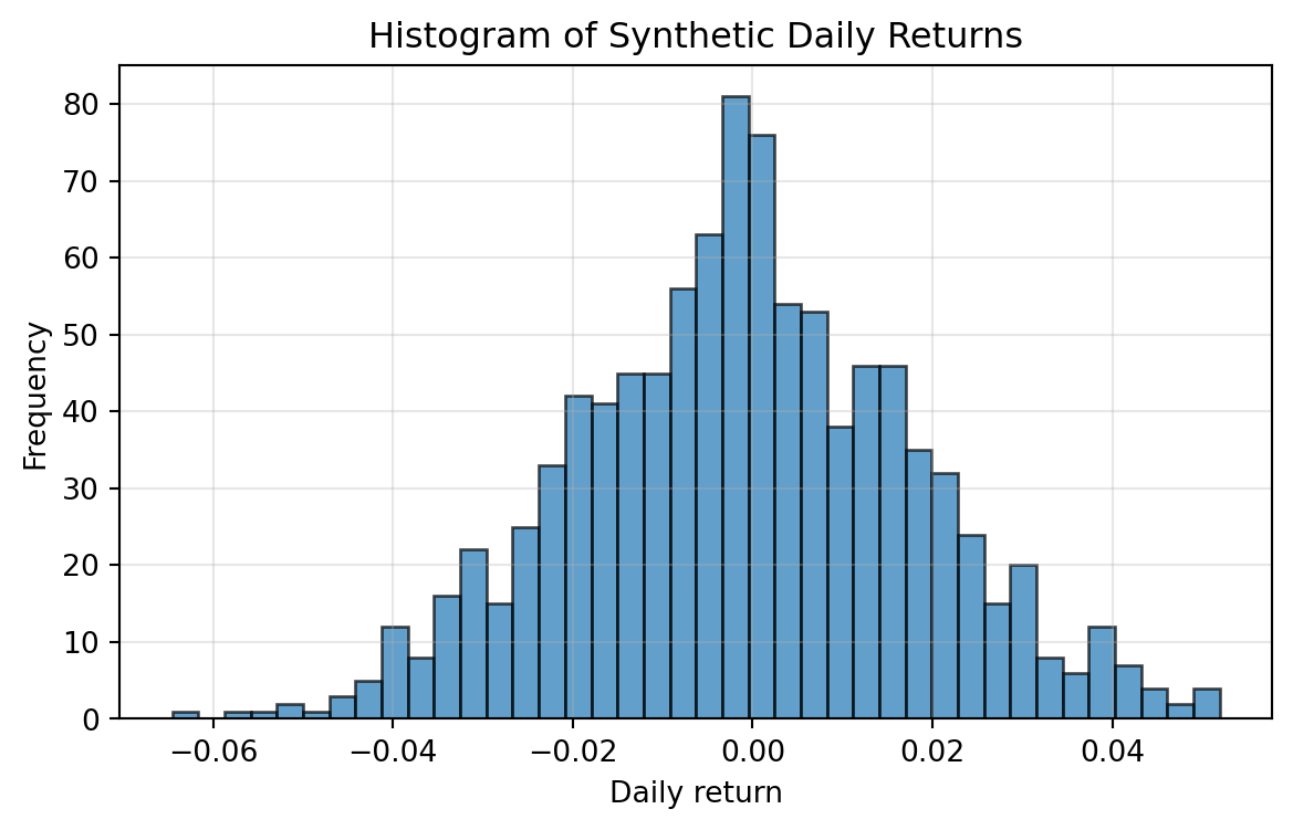
42.3 Multiple lines
x = np.linspace(0, 1, 100)
y1 = x
y2 = x**2
y3 = np.sqrt(x)

plt.figure(figsize=(7, 4))
plt.plot(x, y1, label="linear")
plt.plot(x, y2, label="quadratic")
plt.plot(x, y3, label="square root")
plt.xlabel("x")
plt.ylabel("value")
plt.title("Example of Multiple Lines")
plt.legend()
plt.grid(True, alpha=0.3)
plt.show()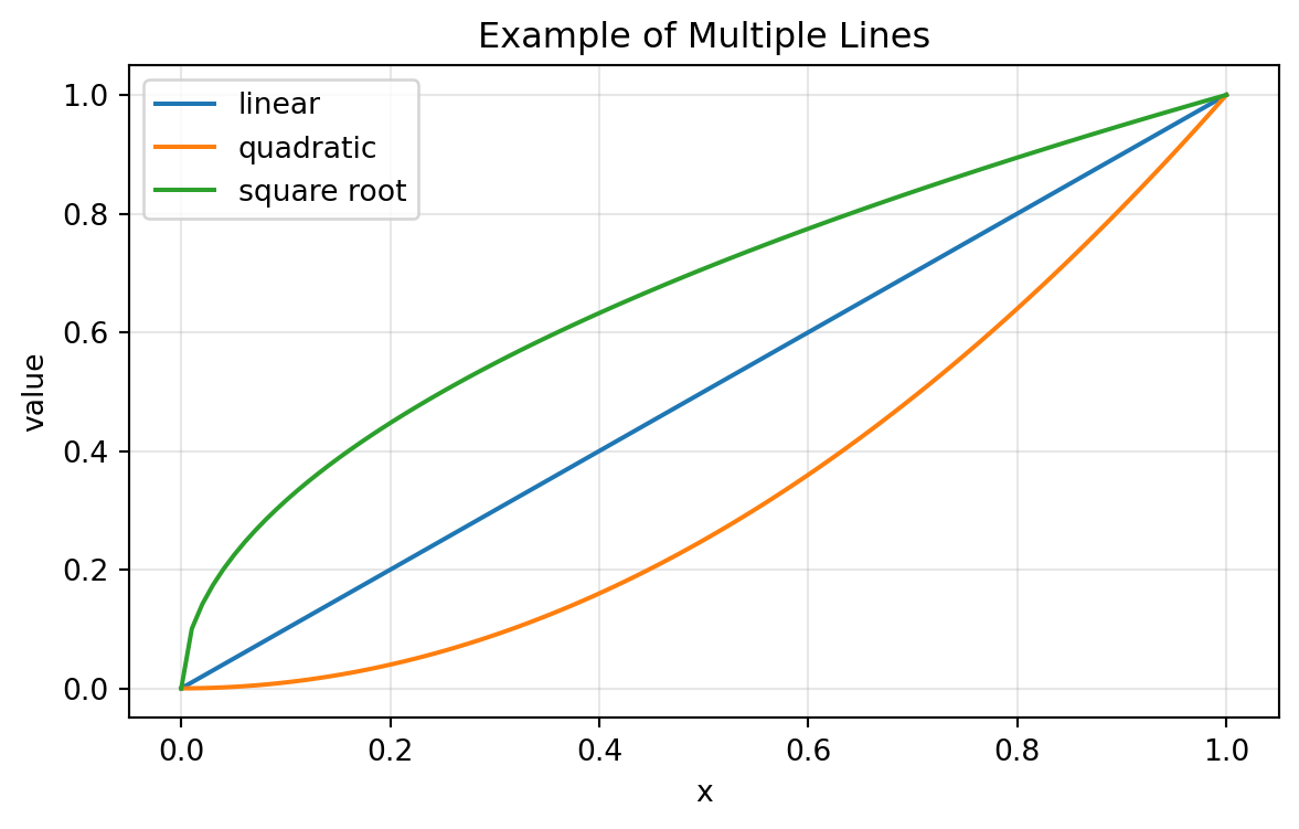
43 Core Financial Calculations
43.1 Simple and log returns
Simple return:
\[ R_t = \frac{S_t}{S_{t-1}} - 1. \]
Log return:
\[ r_t = \log S_t - \log S_{t-1}. \]
def simple_returns_from_prices(prices):
    prices = np.asarray(prices, dtype=float)
    return prices[1:] / prices[:-1] - 1


def log_returns_from_prices(prices):
    prices = np.asarray(prices, dtype=float)
    return np.diff(np.log(prices))

prices = np.array([100, 102, 101, 105])
simple_returns_from_prices(prices), log_returns_from_prices(prices)
(array([ 0.02 , -0.00980392, 0.03960396]),
array([ 0.01980263, -0.0098523 , 0.03883983]))43.2 Compounding
If the continuously compounded rate is \(r\), then the value of one dollar after time \(T\) is
\[ e^{rT}. \]
The discount factor is
\[ D(0,T)=e^{-rT}. \]
def discount_factor(r, T):
    return np.exp(-r * T)


def future_value_continuous(amount, r, T):
    return amount * np.exp(r * T)

r = 0.05
T = 2
amount = 100

discount_factor(r, T), future_value_continuous(amount, r, T)
(0.9048374180359595, 110.51709180756477)43.3 Portfolio return
For weights \(w_1,\ldots,w_d\) and asset returns \(R_1,\ldots,R_d\),
\[ R_p = \sum_{i=1}^d w_i R_i. \]
weights = np.array([0.5, 0.3, 0.2])
asset_returns = np.array([0.01, -0.005, 0.02])
portfolio_return = weights @ asset_returns
portfolio_return0.00750000000000000144 Binomial Models
44.1 One-step binomial price
In a one-period model,
\[ S_u = uS_0, \qquad S_d = dS_0. \]
With risk-free growth factor \(R=1+r\Delta t\), the risk-neutral probability is
\[ q = \frac{R-d}{u-d}. \]
The no-arbitrage condition is
\[ d < R < u. \]
def one_step_binomial_call(S0, K, R, u, d):
    q = (R - d) / (u - d)
    payoff_u = max(u * S0 - K, 0)
    payoff_d = max(d * S0 - K, 0)
    price = (q * payoff_u + (1 - q) * payoff_d) / R
    return price

one_step_binomial_call(S0=100, K=100, R=1.02, u=1.15, d=0.90)7.05882352941176144.2 Multi-step CRR tree
For the Cox–Ross–Rubinstein model,
\[ u = e^{\sigma \sqrt{\Delta t}}, \qquad d = e^{-\sigma \sqrt{\Delta t}}. \]
def crr_european_option(S0, K, r, sigma, T, N, option_type="call"):
    dt = T / N
    u = np.exp(sigma * np.sqrt(dt))
    d = 1 / u
    R = np.exp(r * dt)
    q = (R - d) / (u - d)

    j = np.arange(N + 1)
    ST = S0 * (u ** j) * (d ** (N - j))

    if option_type == "call":
        values = np.maximum(ST - K, 0)
    elif option_type == "put":
        values = np.maximum(K - ST, 0)
    else:
        raise ValueError("option_type must be 'call' or 'put'")

    for n in range(N - 1, -1, -1):
        values = (q * values[1:] + (1 - q) * values[:-1]) / R

    return values[0]

crr_european_option(100, 100, 0.05, 0.20, 1.0, 100, "call")10.43061166224918445 Black–Scholes Formulas
Under the risk-neutral Black–Scholes model,
\[ dS_t = rS_t\,dt + \sigma S_t\,dW_t. \]
The European call price is
\[ C = S_0 N(d_1) - Ke^{-rT}N(d_2), \]
where
\[ d_1 = \frac{\log(S_0/K)+(r+\sigma^2/2)T}{\sigma\sqrt{T}}, \qquad d_2=d_1-\sigma\sqrt{T}. \]
The put price is
\[ P = Ke^{-rT}N(-d_2)-S_0N(-d_1). \]
def bs_d1_d2(S0, K, r, sigma, T):
    if T <= 0 or sigma <= 0:
        raise ValueError("T and sigma must be positive.")
    d1 = (np.log(S0 / K) + (r + 0.5 * sigma**2) * T) / (sigma * np.sqrt(T))
    d2 = d1 - sigma * np.sqrt(T)
    return d1, d2


def bs_call_price(S0, K, r, sigma, T):
    d1, d2 = bs_d1_d2(S0, K, r, sigma, T)
    return S0 * norm.cdf(d1) - K * np.exp(-r * T) * norm.cdf(d2)


def bs_put_price(S0, K, r, sigma, T):
    d1, d2 = bs_d1_d2(S0, K, r, sigma, T)
    return K * np.exp(-r * T) * norm.cdf(-d2) - S0 * norm.cdf(-d1)

bs_call_price(100, 100, 0.05, 0.20, 1.0), bs_put_price(100, 100, 0.05, 0.20, 1.0)
(10.450583572185565, 5.573526022256971)45.1 Greeks
def bs_call_delta(S0, K, r, sigma, T):
    d1, d2 = bs_d1_d2(S0, K, r, sigma, T)
    return norm.cdf(d1)


def bs_put_delta(S0, K, r, sigma, T):
    d1, d2 = bs_d1_d2(S0, K, r, sigma, T)
    return norm.cdf(d1) - 1


def bs_gamma(S0, K, r, sigma, T):
    d1, d2 = bs_d1_d2(S0, K, r, sigma, T)
    return norm.pdf(d1) / (S0 * sigma * np.sqrt(T))


def bs_vega(S0, K, r, sigma, T):
    d1, d2 = bs_d1_d2(S0, K, r, sigma, T)
    return S0 * norm.pdf(d1) * np.sqrt(T)

S0, K, r, sigma, T = 100, 100, 0.05, 0.20, 1.0
bs_call_delta(S0, K, r, sigma, T), bs_gamma(S0, K, r, sigma, T), bs_vega(S0, K, r, sigma, T)
(0.6368306511756191, 0.018762017345846895, 37.52403469169379)46 Implied Volatility
Given a market call price \(C_{mkt}\), the implied volatility is the value of \(\sigma\) satisfying
\[ C_{BS}(S_0,K,r,\sigma,T)=C_{mkt}. \]
def implied_vol_call(price, S0, K, r, T, low=1e-6, high=5.0):
    intrinsic_lower = max(S0 - K * np.exp(-r * T), 0)
    upper = S0

    if price < intrinsic_lower - 1e-10 or price > upper + 1e-10:
        return np.nan

    def objective(sigma):
        return bs_call_price(S0, K, r, sigma, T) - price

    try:
        return brentq(objective, low, high)
    except ValueError:
        return np.nan

true_sigma = 0.25
market_price = bs_call_price(100, 105, 0.03, true_sigma, 1.0)
implied_vol_call(market_price, 100, 105, 0.03, 1.0)0.2499999999999995347 Monte Carlo Simulation
47.1 Brownian motion
Brownian increments satisfy
\[ \Delta W_i \sim N(0,\Delta t). \]
def simulate_brownian_paths(T=1.0, N=252, M=5, seed=1):
    rng = np.random.default_rng(seed)
    dt = T / N
    dW = rng.normal(0, np.sqrt(dt), size=(M, N))
    W = np.cumsum(dW, axis=1)
    W = np.column_stack([np.zeros(M), W])
    time_grid = np.linspace(0, T, N + 1)
    return time_grid, W

time_grid, W = simulate_brownian_paths(M=3)
W[:, :5]
array([[ 0. , 0.02176976, 0.07352684, 0.09434242, 0.01225123],
[ 0. , 0.01548223, -0.03155248, 0.0112041 , -0.01839683],
[ 0. , -0.07564727, -0.00570067, -0.06164476, -0.01952336]])47.2 Geometric Brownian motion
The exact solution of
\[ dS_t=\mu S_t\,dt+\sigma S_t\,dW_t \]
is
\[ S_t = S_0 \exp\left((\mu-\sigma^2/2)t + \sigma W_t\right). \]
def simulate_gbm_paths(S0=100, mu=0.05, sigma=0.20, T=1.0, N=252, M=10000, seed=1):
    rng = np.random.default_rng(seed)
    dt = T / N
    Z = rng.normal(size=(M, N))
    increments = (mu - 0.5 * sigma**2) * dt + sigma * np.sqrt(dt) * Z
    log_paths = np.cumsum(increments, axis=1)
    log_paths = np.column_stack([np.zeros(M), log_paths])
    S = S0 * np.exp(log_paths)
    time_grid = np.linspace(0, T, N + 1)
    return time_grid, S

time_grid, S_paths = simulate_gbm_paths(M=3, seed=2)
S_paths[:, :5]
array([[100. , 100.25040262, 99.60417871, 99.0989707 ,
96.10857141],
[100. , 98.53475765, 97.96576 , 97.03649864,
95.5336124 ],
[100. , 101.77268967, 101.20206936, 102.1269847 ,
103.16324612]])47.3 Monte Carlo option price
Under the risk-neutral measure,
\[ V_0 = e^{-rT}E_Q[\text{payoff}(S_T)]. \]
def mc_european_call(S0, K, r, sigma, T, M=100000, seed=1):
    rng = np.random.default_rng(seed)
    Z = rng.normal(size=M)
    ST = S0 * np.exp((r - 0.5 * sigma**2) * T + sigma * np.sqrt(T) * Z)
    payoff = np.maximum(ST - K, 0)
    discounted = np.exp(-r * T) * payoff
    price = discounted.mean()
    se = discounted.std(ddof=1) / np.sqrt(M)
    return price, se

price, se = mc_european_call(100, 100, 0.05, 0.20, 1.0)
price, se
(10.357757644151459, 0.046422222989210477)A 95 percent confidence interval is approximately
\[ \hat V \pm 1.96\,\text{SE}. \]
price - 1.96 * se, price + 1.96 * se(10.266770087092606, 10.448745201210311)48 Variance Reduction
48.1 Antithetic variables
Use both \(Z\) and \(-Z\) to reduce simulation noise.
def mc_call_antithetic(S0, K, r, sigma, T, M=100000, seed=1):
    rng = np.random.default_rng(seed)
    half = M // 2
    Z = rng.normal(size=half)
    Z_full = np.concatenate([Z, -Z])
    ST = S0 * np.exp((r - 0.5 * sigma**2) * T + sigma * np.sqrt(T) * Z_full)
    payoff = np.maximum(ST - K, 0)
    discounted = np.exp(-r * T) * payoff
    return discounted.mean(), discounted.std(ddof=1) / np.sqrt(len(discounted))

mc_call_antithetic(100, 100, 0.05, 0.20, 1.0)
(10.401421575814576, 0.04638684662155947)48.2 Control variates
If \(X\) is the payoff to price and \(Y\) has known mean \(E[Y]\), then
\[ X^{cv} = X - b(Y-E[Y]). \]
The optimal coefficient is approximately
\[ b^* = \frac{\operatorname{Cov}(X,Y)}{\operatorname{Var}(Y)}. \]
def control_variate_estimator(X, Y, EY):
    cov_xy = np.cov(X, Y, ddof=1)[0, 1]
    var_y = np.var(Y, ddof=1)
    b = cov_xy / var_y
    X_cv = X - b * (Y - EY)
    return X_cv.mean(), X_cv.std(ddof=1) / np.sqrt(len(X_cv)), b
49 Path-Dependent Options
49.1 Asian option payoff
Arithmetic Asian call:
\[ \text{payoff}=\max\left(\frac{1}{N}\sum_{i=1}^N S_{t_i}-K,0\right). \]
def asian_call_payoff(S_paths, K):
    average_price = S_paths[:, 1:].mean(axis=1)
    return np.maximum(average_price - K, 0)

_, S_paths = simulate_gbm_paths(S0=100, mu=0.05, sigma=0.20, T=1.0, N=252, M=10000, seed=3)
payoff = asian_call_payoff(S_paths, K=100)
np.exp(-0.05) * payoff.mean()5.62519285677176349.2 Barrier option payoff
Up-and-out call:
\[ \text{payoff}=\max(S_T-K,0)\mathbf{1}_{\max_t S_t < B}. \]
def up_and_out_call_payoff(S_paths, K, B):
    ST = S_paths[:, -1]
    knocked_out = S_paths.max(axis=1) >= B
    return np.maximum(ST - K, 0) * (~knocked_out)

payoff = up_and_out_call_payoff(S_paths, K=100, B=130)
np.exp(-0.05) * payoff.mean()3.426452324166095650 Finite Difference Helpers
Many PDE methods use grids.
S_max = 300
M = 100
N = 100
T = 1.0

dS = S_max / M
dt = T / N
S_grid = np.linspace(0, S_max, M + 1)
time_grid = np.linspace(0, T, N + 1)

S_grid[:5], time_grid[:5]
(array([ 0., 3., 6., 9., 12.]), array([0. , 0.01, 0.02, 0.03, 0.04]))A terminal payoff for a European call is:
K = 100
payoff = np.maximum(S_grid - K, 0)
payoff[:10]
array([0., 0., 0., 0., 0., 0., 0., 0., 0., 0.])50.1 Thomas algorithm for tridiagonal systems
Finite-difference schemes often require solving tridiagonal systems.
def thomas_algorithm(a, b, c, d):
    """Solve a tridiagonal linear system.

    a: lower diagonal, length n-1
    b: main diagonal, length n
    c: upper diagonal, length n-1
    d: right-hand side, length n
    """
    a = np.asarray(a, dtype=float)
    b = np.asarray(b, dtype=float)
    c = np.asarray(c, dtype=float)
    d = np.asarray(d, dtype=float)

    n = len(b)
    cp = np.zeros(n - 1)
    dp = np.zeros(n)

    cp[0] = c[0] / b[0]
    dp[0] = d[0] / b[0]

    for i in range(1, n - 1):
        denom = b[i] - a[i - 1] * cp[i - 1]
        cp[i] = c[i] / denom
        dp[i] = (d[i] - a[i - 1] * dp[i - 1]) / denom

    dp[n - 1] = (d[n - 1] - a[n - 2] * dp[n - 2]) / (b[n - 1] - a[n - 2] * cp[n - 2])

    x = np.zeros(n)
    x[-1] = dp[-1]
    for i in range(n - 2, -1, -1):
        x[i] = dp[i] - cp[i] * x[i + 1]

    return x
51 Stochastic Calculus by Simulation
51.1 Quadratic variation
For Brownian motion,
\[ \sum_i (W_{t_{i+1}}-W_{t_i})^2 \to T. \]
def brownian_quadratic_variation(T=1.0, N=1000, M=5000, seed=1):
    rng = np.random.default_rng(seed)
    dt = T / N
    dW = rng.normal(0, np.sqrt(dt), size=(M, N))
    qv = np.sum(dW**2, axis=1)
    return qv

qv = brownian_quadratic_variation()
qv.mean(), qv.std(ddof=1)
(0.999811582097473, 0.04429882086432296)51.2 Ito integral approximation
The Ito integral uses left-endpoint sums:
\[ \int_0^T H_t\,dW_t \approx \sum_i H_{t_i}(W_{t_{i+1}}-W_{t_i}). \]
def ito_integral_W_dW(T=1.0, N=1000, M=5000, seed=1):
    rng = np.random.default_rng(seed)
    dt = T / N
    dW = rng.normal(0, np.sqrt(dt), size=(M, N))
    W_left = np.column_stack([np.zeros(M), np.cumsum(dW, axis=1)[:, :-1]])
    integral = np.sum(W_left * dW, axis=1)
    W_T = np.sum(dW, axis=1)
    exact = 0.5 * (W_T**2 - T)
    return integral, exact

integral, exact = ito_integral_W_dW()
np.mean(integral - exact), np.std(integral - exact, ddof=1)
(9.420895126346042e-05, 0.02214941043216151)52 Change of Measure
If
\[ dS_t = \mu S_t\,dt + \sigma S_t\,dW_t^P, \]
then the market price of risk is
\[ \theta = \frac{\mu-r}{\sigma}. \]
A risk-neutral Brownian motion can be written as
\[ W_t^Q = W_t^P + \theta t. \]
The terminal likelihood ratio for changing from \(P\) to \(Q\) is
\[ Z_T = \exp\left(-\theta W_T^P - \frac12\theta^2 T\right). \]
def girsanov_density_terminal(W_T_P, theta, T):
    return np.exp(-theta * W_T_P - 0.5 * theta**2 * T)

T = 1.0
mu = 0.10
r = 0.04
sigma = 0.20
theta = (mu - r) / sigma

rng = np.random.default_rng(11)
W_T_P = rng.normal(0, np.sqrt(T), size=100000)
Z_T = girsanov_density_terminal(W_T_P, theta, T)
Z_T.mean()1.000164196219111753 Fixed Income Helpers
53.1 Discount factor and zero rate
If \(P(0,T)\) is the discount factor, the continuously compounded zero rate is
\[ y(0,T) = -\frac{1}{T}\log P(0,T). \]
def zero_rate_from_discount(P, T):
    return -np.log(P) / T


def discount_from_zero_rate(y, T):
    return np.exp(-y * T)

P = discount_from_zero_rate(0.04, 5)
y = zero_rate_from_discount(P, 5)
P, y
(0.8187307530779818, 0.04000000000000001)53.2 Bond pricing from cash flows
def bond_price_from_curve(times, cashflows, zero_rate_func):
    times = np.asarray(times, dtype=float)
    cashflows = np.asarray(cashflows, dtype=float)
    discounts = np.exp(-np.array([zero_rate_func(t) * t for t in times]))
    return np.sum(cashflows * discounts)


def flat_zero_rate(t):
    return 0.04

times = np.array([1, 2, 3, 4, 5])
cashflows = np.array([3, 3, 3, 3, 103])
bond_price_from_curve(times, cashflows, flat_zero_rate)95.1981776006991153.3 Duration and convexity
Macaulay duration:
\[ D_M = \frac{\sum_i t_i PV(C_i)}{\sum_i PV(C_i)}. \]
def macaulay_duration(times, cashflows, y):
    times = np.asarray(times, dtype=float)
    cashflows = np.asarray(cashflows, dtype=float)
    discounts = np.exp(-y * times)
    price = np.sum(cashflows * discounts)
    return np.sum(times * cashflows * discounts) / price

macaulay_duration(times, cashflows, 0.04)4.70886549435053954 Short-Rate Models
54.1 Vasicek simulation
The Vasicek model is
\[ dr_t = \kappa(\theta-r_t)dt + \sigma dW_t. \]
def simulate_vasicek(r0, kappa, theta, sigma, T, N, M, seed=1):
    rng = np.random.default_rng(seed)
    dt = T / N
    rates = np.zeros((M, N + 1))
    rates[:, 0] = r0

    exp_kdt = np.exp(-kappa * dt)
    mean_coeff = theta * (1 - exp_kdt)
    var = sigma**2 * (1 - np.exp(-2 * kappa * dt)) / (2 * kappa)

    for n in range(N):
        Z = rng.normal(size=M)
        rates[:, n + 1] = rates[:, n] * exp_kdt + mean_coeff + np.sqrt(var) * Z

    time_grid = np.linspace(0, T, N + 1)
    return time_grid, rates

time_grid, rates = simulate_vasicek(0.03, 1.2, 0.04, 0.015, 5.0, 250, 3, seed=1)
rates[:, :5]
array([[0.03 , 0.03096153, 0.0284443 , 0.02759282, 0.02850358],
[0.03 , 0.03195935, 0.03404776, 0.03540701, 0.0355755 ],
[0.03 , 0.03092978, 0.03208053, 0.03303252, 0.03434372]])54.2 CIR simulation with full truncation Euler
The CIR model is
\[ dr_t = \kappa(\theta-r_t)dt + \sigma\sqrt{r_t}\,dW_t. \]
def simulate_cir_full_truncation(r0, kappa, theta, sigma, T, N, M, seed=1):
    rng = np.random.default_rng(seed)
    dt = T / N
    rates = np.zeros((M, N + 1))
    rates[:, 0] = r0

    for n in range(N):
        r_plus = np.maximum(rates[:, n], 0)
        Z = rng.normal(size=M)
        rates[:, n + 1] = rates[:, n] + kappa * (theta - r_plus) * dt + sigma * np.sqrt(r_plus) * np.sqrt(dt) * Z
        rates[:, n + 1] = np.maximum(rates[:, n + 1], 0)

    time_grid = np.linspace(0, T, N + 1)
    return time_grid, rates

time_grid, cir_rates = simulate_cir_full_truncation(0.03, 1.2, 0.04, 0.15, 5.0, 250, 3, seed=2)
cir_rates[:, :5]
array([[0.03 , 0.03093463, 0.02204301, 0.02144906, 0.02017367],
[0.03 , 0.0283193 , 0.03502429, 0.03821572, 0.04231245],
[0.03 , 0.02872231, 0.03310641, 0.03435727, 0.03327158]])55 Portfolio Optimization
For expected return vector \(\mu\), covariance matrix \(\Sigma\), and weights \(w\),
\[ E[R_p]=w^T\mu, \qquad \operatorname{Var}(R_p)=w^T\Sigma w. \]
def portfolio_mean(w, mu):
    return float(w @ mu)


def portfolio_vol(w, Sigma):
    return float(np.sqrt(w @ Sigma @ w))


def portfolio_sharpe(w, mu, Sigma, rf=0.0):
    vol = portfolio_vol(w, Sigma)
    return (portfolio_mean(w, mu) - rf) / vol

mu = np.array([0.08, 0.10, 0.06])
Sigma = np.array([
    [0.04, 0.018, 0.010],
    [0.018, 0.09, 0.015],
    [0.010, 0.015, 0.025]
])
w = np.array([0.4, 0.4, 0.2])

portfolio_mean(w, mu), portfolio_vol(w, Sigma), portfolio_sharpe(w, mu, Sigma, rf=0.03)
(0.084, 0.17765134392961965, 0.3039661778263454)55.1 Long-only minimum variance portfolio
def min_variance_long_only(Sigma):
    n = Sigma.shape[0]
    x0 = np.ones(n) / n
    bounds = [(0, 1) for _ in range(n)]
    constraints = ({"type": "eq", "fun": lambda w: np.sum(w) - 1})

    result = minimize(lambda w: w @ Sigma @ w, x0=x0, bounds=bounds, constraints=constraints)
    if not result.success:
        raise RuntimeError(result.message)
    return result.x

w_min = min_variance_long_only(Sigma)
w_min, portfolio_vol(w_min, Sigma)
(array([0.31279637, 0.05130952, 0.63589411]), 0.14069237835825074)56 Factor Models
A linear factor model has the form
\[ R_i-r_f = \alpha_i + \beta_{i1}F_1+\cdots+\beta_{ik}F_k + \epsilon_i. \]
56.1 Ordinary least squares with NumPy
def ols_fit(y, X, add_intercept=True):
    y = np.asarray(y, dtype=float)
    X = np.asarray(X, dtype=float)
    if add_intercept:
        X_design = np.column_stack([np.ones(len(X)), X])
    else:
        X_design = X
    beta_hat, residuals, rank, s = np.linalg.lstsq(X_design, y, rcond=None)
    fitted = X_design @ beta_hat
    resid = y - fitted
    return beta_hat, fitted, resid

rng = np.random.default_rng(4)
T_obs = 250
market = rng.normal(0.0005, 0.01, size=T_obs)
asset = 0.0001 + 1.3 * market + rng.normal(0, 0.008, size=T_obs)

coef, fitted, resid = ols_fit(asset, market)
coef
array([-1.98241768e-04, 1.21152131e+00])The first coefficient is alpha. The second coefficient is beta.
57 Risk Measures
57.1 Historical VaR and Expected Shortfall
Let \(L\) denote portfolio loss. The level \(\alpha\) Value at Risk is approximately the \(\alpha\) quantile of losses.
Expected Shortfall is the average loss beyond VaR.
def historical_var(losses, alpha=0.99):
    return np.quantile(losses, alpha)


def historical_es(losses, alpha=0.99):
    var = historical_var(losses, alpha)
    return losses[losses >= var].mean()

rng = np.random.default_rng(5)
portfolio_returns = rng.normal(0.0003, 0.015, size=2000)
losses = -portfolio_returns
historical_var(losses, 0.99), historical_es(losses, 0.99)
(0.03485729700101692, 0.03889603568334813)57.2 Normal VaR and Expected Shortfall
If losses are approximately normal with mean \(m\) and standard deviation \(s\), then
\[ VaR_\alpha = m + s\Phi^{-1}(\alpha), \]
and
\[ ES_\alpha = m + s\frac{\phi(\Phi^{-1}(\alpha))}{1-\alpha}. \]
def normal_var_es(losses, alpha=0.99):
    m = np.mean(losses)
    s = np.std(losses, ddof=1)
    z = norm.ppf(alpha)
    var = m + s * z
    es = m + s * norm.pdf(z) / (1 - alpha)
    return var, es

normal_var_es(losses, 0.99)
(0.033575060206886054, 0.038562267361719846)58 Calibration Patterns
Many calibration problems have the form:
\[ \min_\theta \sum_i \left(m_i(\theta)-q_i\right)^2, \]
where \(q_i\) are market quotes and \(m_i(\theta)\) are model prices or model-implied quantities.
def calibrate_constant_volatility(option_quotes, S0, r):
    """Calibrate one Black--Scholes volatility to multiple call prices.

    option_quotes should be a DataFrame with columns K, T, price.
    """
    def objective(x):
        sigma = x[0]
        if sigma <= 0:
            return 1e10
        errors = []
        for _, row in option_quotes.iterrows():
            model_price = bs_call_price(S0, row["K"], r, sigma, row["T"])
            errors.append(model_price - row["price"])
        return np.mean(np.array(errors)**2)

    result = minimize(objective, x0=np.array([0.20]), bounds=[(1e-4, 3.0)])
    return result.x[0], result.fun

quotes = pd.DataFrame({
    "K": [90, 100, 110],
    "T": [1.0, 1.0, 1.0],
    "price": [bs_call_price(100, 90, 0.03, 0.24, 1.0),
              bs_call_price(100, 100, 0.03, 0.20, 1.0),
              bs_call_price(100, 110, 0.03, 0.22, 1.0)]
})

calibrate_constant_volatility(quotes, S0=100, r=0.03)
(0.21724381291044406, 0.3188809895799794)59 Numerical Stability and Good Habits
59.1 Use functions
Instead of writing the same code repeatedly, define functions. This makes the notebook easier to read and debug.
59.2 Use seeds for reproducibility
rng = np.random.default_rng(123)59.3 Check units
Daily, monthly, and annual quantities must be handled carefully. For example, if the annual volatility is \(\sigma_{ann}\), then daily volatility with 252 trading days is approximately
\[ \sigma_{daily}=\frac{\sigma_{ann}}{\sqrt{252}}. \]
sigma_annual = 0.20
sigma_daily = sigma_annual / np.sqrt(252)
sigma_daily0.0125988157669742459.4 Check no-arbitrage bounds
For a European call with no dividends,
\[ \max(S_0-Ke^{-rT},0) \le C \le S_0. \]
def call_no_arbitrage_bounds(S0, K, r, T):
    lower = max(S0 - K * np.exp(-r * T), 0)
    upper = S0
    return lower, upper

call_no_arbitrage_bounds(100, 105, 0.03, 1.0)
(0, 100)For a European put,
\[ \max(Ke^{-rT}-S_0,0) \le P \le Ke^{-rT}. \]
def put_no_arbitrage_bounds(S0, K, r, T):
    lower = max(K * np.exp(-r * T) - S0, 0)
    upper = K * np.exp(-r * T)
    return lower, upper

put_no_arbitrage_bounds(100, 105, 0.03, 1.0)
(1.896781022593359, 101.89678102259336)59.5 Use numerical tolerances
Floating-point arithmetic is approximate. Instead of testing exact equality, use np.isclose.
np.isclose(0.1 + 0.2, 0.3)True60 Common Debugging Tips
60.1 Shape errors
Many mistakes come from mismatched array shapes.
A = np.ones((3, 2))
b = np.ones(2)
A @ b
array([2., 2., 2.])Check shapes with:
A.shape, b.shape((3, 2), (2,))60.2 NaN values
Use these commands to check for missing or invalid values:
x = np.array([1.0, np.nan, 2.0])
np.isnan(x)
array([False, True, False])np.nanmean(x)1.560.3 Slow Monte Carlo cells
If a Monte Carlo cell is slow, reduce the number of paths first:
M = 5000   # faster for debugging
# M = 100000  # use later for more accuracy
60.4 Plotting too many paths
Simulate many paths, but plot only a few.
time_grid, S_paths = simulate_gbm_paths(M=20000, seed=9)

plt.figure(figsize=(7, 4))
for i in range(10):
    plt.plot(time_grid, S_paths[i], alpha=0.8)
plt.xlabel("Time")
plt.ylabel("Stock price")
plt.title("Plot Only a Few Simulated Paths")
plt.grid(True, alpha=0.3)
plt.show()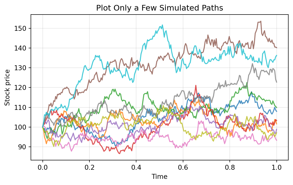
61 Lab-by-Lab Python Skills
| Lab | Main Python skills |
|---|---|
| 1 | arrays, returns, compounding, one-period payoff calculations |
| 2 | backward induction, binomial trees, vectorized terminal payoffs |
| 3 | Brownian motion, GBM simulation, Monte Carlo confidence intervals |
| 4 | Black–Scholes functions, Greeks, finite-difference checks, hedging simulation |
| 5 | root finding, implied volatility, smile fitting |
| 6 | variance reduction, repeated Monte Carlo comparisons |
| 7 | path-dependent payoffs, Asian/barrier/lookback simulation |
| 8 | PDE grids, tridiagonal systems, finite-difference schemes |
| 9 | Ito sums, quadratic variation, stochastic calculus simulations |
| 10 | likelihood ratios, change of measure, martingale checks |
| 11 | bond cash flows, duration, convexity, curve bootstrapping |
| 12 | short-rate simulations, affine bond pricing, calibration |
| 13 | forward-rate curves, HJM drift, PCA of yield changes |
| 14 | covariance matrices, constrained optimization, efficient frontiers |
| 15 | regression, CAPM, factor exposures, risk decomposition |
| 16 | VaR, Expected Shortfall, rolling forecasts, backtesting |
| 17 | stochastic volatility, correlated Brownian motion, Heston smile calibration |
| 18 | integrated workflow: calibration, hedging, portfolio risk |
62 Recommended Coding Style for Students
Use clear variable names:
S0 = 100       # initial stock price
K = 100        # strike price
r = 0.05       # continuously compounded risk-free rate
sigma = 0.20   # annual volatility
T = 1.0        # maturity in years
Avoid unexplained magic numbers. Add comments when a parameter has financial meaning.
Write small functions and test them with simple inputs before using them in large simulations.
63 Minimal Template for a New Lab Experiment
# 1. Import packages
import numpy as np
import pandas as pd
import matplotlib.pyplot as plt
from scipy.stats import norm

# 2. Set parameters
S0 = 100
K = 100
r = 0.05
sigma = 0.20
T = 1.0
M = 50000
seed = 2026

# 3. Simulate or compute
price, se = mc_european_call(S0, K, r, sigma, T, M=M, seed=seed)

# 4. Summarize results
summary = pd.DataFrame({
    "quantity": ["Monte Carlo price", "standard error"],
    "value": [price, se]
})
summary| quantity | value | |
|---|---|---|
| 0 | Monte Carlo price | 10.441497 |
| 1 | standard error | 0.065636 |
64 Final Advice
The purpose of Python in this book is not only to produce numbers. The deeper purpose is to make mathematical finance visible:
- simulate the objects defined in theory;
- test identities numerically;
- compare models;
- understand approximation error;
- see the effect of parameters;
- connect pricing, hedging, calibration, and risk.
Students should treat each notebook as a mathematical laboratory. Run the code, change the assumptions, and ask what remains stable and what changes.