---
title: "Chapter 9. Markov Chains and Regime Models"
---
::: {.chapter-objectives}
## Learning Goals
By the end of this chapter, students should be able to:
- define a finite-state Markov chain and interpret its transition matrix;
- compute multi-step transition probabilities using matrix powers;
- distinguish row-vector and column-vector conventions for probability distributions;
- derive and compute stationary distributions;
- explain recurrence, transience, irreducibility, periodicity, and long-run behavior in finite chains;
- use Markov chains to model financial regimes such as bull, bear, crisis, and recovery states;
- build Markov reward models for cumulative returns and risk quantities;
- understand the basic structure of hidden Markov models for unobserved regimes;
- implement simulation, filtering, stationary calculations, and regime-switching return models in Python;
- use AI tools to audit transition matrices, explain model assumptions, and test Markov-chain code.
:::
::: {.hero-box}
Financial data often looks different in different market environments. A calm expansion, a high-volatility crisis, and a recovery period do not have the same return distribution. A Markov chain gives a clean mathematical way to model such changing environments.
The central object is a transition matrix $P$. If $X_t$ is the regime at time $t$, then
$$
P_{ij}=\mathbb P(X_{t+1}=j\mid X_t=i).
$$
The Markov assumption says that the next regime depends on the present regime, not on the entire past. This chapter develops the linear algebra and probability behind Markov chains and shows how they enter mathematical finance.
:::
## 9.1 Why Markov Chains Appear in Finance
Many financial quantities have persistence. Volatility clusters. Interest rates move through high-rate and low-rate phases. Credit quality changes through rating transitions. Equity markets may spend long periods in calm growth and shorter periods in crisis. These examples suggest that the distribution of tomorrow's outcome depends on the current environment.
A regime model introduces a finite set of states such as
$$
\mathcal S=\{\text{bear},\text{bull}\}
$$
or
$$
\mathcal S=\{\text{expansion},\text{slowdown},\text{recession},\text{recovery}\}.
$$
The regime process $(X_t)_{t\ge 0}$ is modeled as a Markov chain. Conditional on the regime, returns may have different means, volatilities, or tail behavior. For example,
$$
R_{t+1}\mid X_t=i \sim N(\mu_i,\sigma_i^2).
$$
This is not yet a complete asset-pricing model. It is a probabilistic model for state evolution and data generation. Later chapters will connect such models with pricing measures, stochastic processes, and risk management.
::: {.callout-note}
## Mathematical theme
A finite Markov chain is probability plus linear algebra. Probability distributions are vectors, transition laws are matrices, and long-run behavior is controlled by eigenvectors and eigenvalues.
:::
## 9.2 Finite-State Markov Chains
Let
$$
\mathcal S=\{1,2,\ldots,m\}
$$
be a finite state space. A stochastic process $(X_t)_{t=0,1,2,\ldots}$ with values in $\mathcal S$ is a Markov chain if the conditional distribution of the next state depends only on the current state.
::: {.definition}
### Definition 9.1: Markov property
A discrete-time process $(X_t)$ is a Markov chain if for every $t\ge 0$ and every sequence of states $i_0,\ldots,i_t,j$ with positive conditioning probability,
$$
\mathbb P(X_{t+1}=j\mid X_t=i_t,X_{t-1}=i_{t-1},\ldots,X_0=i_0)
=
\mathbb P(X_{t+1}=j\mid X_t=i_t).
$$
:::
If the transition probabilities do not depend on $t$, the chain is time-homogeneous.
::: {.definition}
### Definition 9.2: Transition matrix
For a time-homogeneous finite Markov chain, the transition matrix is the $m\times m$ matrix
$$
P=(P_{ij})_{i,j=1}^m,
\qquad
P_{ij}=\mathbb P(X_{t+1}=j\mid X_t=i).
$$
Each row is a probability distribution, so
$$
P_{ij}\ge 0,
\qquad
\sum_{j=1}^m P_{ij}=1.
$$
Such a matrix is called row-stochastic.
:::
Throughout this chapter, probability distributions are row vectors. If
$$
\alpha_t=(\mathbb P(X_t=1),\ldots,\mathbb P(X_t=m)),
$$
then the one-step update is
$$
\alpha_{t+1}=\alpha_t P.
$$
The $n$-step distribution is therefore
$$
\alpha_n=\alpha_0P^n.
$$
::: {.warning}
Some books use column probability vectors and write $\alpha_{t+1}=P^\top\alpha_t$. Both conventions are valid, but mixing them creates many mistakes. In this chapter, distributions are row vectors and transition matrices act on the right.
:::
## 9.3 A Two-State Bull--Bear Model
Consider two regimes:
$$
1=\text{bear},
\qquad
2=\text{bull}.
$$
A simple transition matrix is
$$
P=
\begin{pmatrix}
0.80 & 0.20\\
0.10 & 0.90
\end{pmatrix}.
$$
The interpretation is:
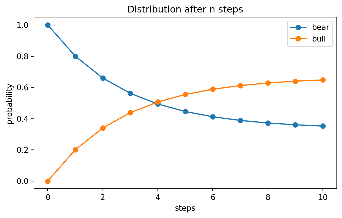
- if the market is currently bear, it remains bear with probability $0.80$ and switches to bull with probability $0.20$;
- if the market is currently bull, it switches to bear with probability $0.10$ and remains bull with probability $0.90$.
Suppose the initial distribution is
$$
\alpha_0=(1,0),
$$
meaning that the market starts in the bear state. Then
$$
\alpha_1=\alpha_0P=(0.80,0.20),
$$
and
$$
\alpha_2=\alpha_0P^2=(0.66,0.34).
$$
The distribution gradually moves toward a long-run equilibrium.
::: {.example}
### Example 9.1: Computing a two-step probability
Starting from bear, the probability of being bull after two steps is
$$
\mathbb P(X_2=\text{bull}\mid X_0=\text{bear})
=
(P^2)_{12}.
$$
There are two paths that end in bull:
$$
\text{bear}\to\text{bear}\to\text{bull}
$$
and
$$
\text{bear}\to\text{bull}\to\text{bull}.
$$
Therefore
$$
(P^2)_{12}=0.80\cdot 0.20+0.20\cdot 0.90=0.34.
$$
:::
## 9.4 Interactive Demo: Regime Probabilities Over Time
The following interactive example shows how a two-state Markov chain evolves. The parameters are
$$
P=
\begin{pmatrix}
1-a & a\\
b & 1-b
\end{pmatrix},
$$
where $a$ is the bear-to-bull transition probability and $b$ is the bull-to-bear transition probability.
<div class="interactive-card">
<h3>Explore a two-state Markov chain</h3>
<p>Move the sliders to change transition probabilities. The plot shows how the probability of the bull state changes over time.</p>
<div class="mf-controls">
<label for="mf-ch09-a">bear to bull probability $a$</label>
<input id="mf-ch09-a" type="range" min="0.01" max="0.80" step="0.01" value="0.20">
<span id="mf-ch09-a-val">0.20</span>
</div>
<div class="mf-controls">
<label for="mf-ch09-b">bull to bear probability $b$</label>
<input id="mf-ch09-b" type="range" min="0.01" max="0.80" step="0.01" value="0.10">
<span id="mf-ch09-b-val">0.10</span>
</div>
<div class="mf-controls">
<label for="mf-ch09-p0">initial bull probability</label>
<input id="mf-ch09-p0" type="range" min="0.00" max="1.00" step="0.01" value="0.00">
<span id="mf-ch09-p0-val">0.00</span>
</div>
<div id="mf-ch09-regime-prob-plot" class="plotly-demo"></div>
<div id="mf-ch09-regime-output" class="mf-output"></div>
</div>
<script>
if (window.mfPlotlyReady) {
window.mfPlotlyReady(function() {
var aSlider = document.getElementById("mf-ch09-a");
var bSlider = document.getElementById("mf-ch09-b");
var p0Slider = document.getElementById("mf-ch09-p0");
var aVal = document.getElementById("mf-ch09-a-val");
var bVal = document.getElementById("mf-ch09-b-val");
var p0Val = document.getElementById("mf-ch09-p0-val");
var output = document.getElementById("mf-ch09-regime-output");
var plot = document.getElementById("mf-ch09-regime-prob-plot");
if (!aSlider || !bSlider || !p0Slider || !plot || typeof Plotly === "undefined") return;
function update() {
var a = Number(aSlider.value);
var b = Number(bSlider.value);
var pBull = Number(p0Slider.value);
var pBear = 1 - pBull;
aVal.textContent = a.toFixed(2);
bVal.textContent = b.toFixed(2);
p0Val.textContent = pBull.toFixed(2);
var times = [];
var bull = [];
var stationaryBull = a / (a + b);
for (var t = 0; t <= 40; t++) {
times.push(t);
bull.push(pBull);
var nextBear = pBear * (1 - a) + pBull * b;
var nextBull = pBear * a + pBull * (1 - b);
pBear = nextBear;
pBull = nextBull;
}
var stationaryLine = times.map(function() { return stationaryBull; });
Plotly.newPlot(plot, [
{x: times, y: bull, mode: "lines+markers", name: "Pr(bull at time t)"},
{x: times, y: stationaryLine, mode: "lines", name: "stationary bull probability", line: {dash: "dash"}}
], {
title: "Evolution of Regime Probability",
xaxis: {title: "time t"},
yaxis: {title: "probability", range: [0, 1]},
margin: {l: 55, r: 20, t: 50, b: 50}
}, {responsive: true});
output.innerHTML = "Stationary distribution: bear = " + (b / (a + b)).toFixed(3) + ", bull = " + stationaryBull.toFixed(3) + ".";
}
[aSlider, bSlider, p0Slider].forEach(function(slider) {
slider.addEventListener("input", update);
});
update();
});
}
</script>
The stationary bull probability is
$$
\pi_{\text{bull}}=\frac{a}{a+b}.
$$
The stationary bear probability is
$$
\pi_{\text{bear}}=\frac{b}{a+b}.
$$
These formulas can be derived by solving $\pi=\pi P$ and $\pi_1+\pi_2=1$.
## 9.5 Multi-Step Transition Probabilities
The transition matrix contains one-step probabilities. Multi-step probabilities are obtained by matrix multiplication.
::: {.theorem}
### Theorem 9.1: Chapman--Kolmogorov equations
For a time-homogeneous Markov chain with transition matrix $P$,
$$
\mathbb P(X_{t+n}=j\mid X_t=i)=(P^n)_{ij}.
$$
More generally,
$$
P^{m+n}=P^mP^n.
$$
:::
::: {.proof}
For two steps,
$$
\mathbb P(X_{t+2}=j\mid X_t=i)
=
\sum_{k=1}^m \mathbb P(X_{t+1}=k,X_{t+2}=j\mid X_t=i).
$$
By the product rule and the Markov property,
$$
\mathbb P(X_{t+1}=k,X_{t+2}=j\mid X_t=i)
=
\mathbb P(X_{t+1}=k\mid X_t=i)
\mathbb P(X_{t+2}=j\mid X_{t+1}=k).
$$
Thus
$$
\mathbb P(X_{t+2}=j\mid X_t=i)
=
\sum_{k=1}^m P_{ik}P_{kj}
=(P^2)_{ij}.
$$
The general result follows by induction.
:::
For finance, $P^n$ is important because it gives the distribution of the future regime. For example, if $P$ describes monthly credit-rating transitions, then $P^{12}$ gives one-year transition probabilities under the same monthly transition model.
```{python}
#| label: ch09-transition-powers
#| fig-cap: "Multi-step transition probabilities in a two-state bull--bear model."
import numpy as np
import pandas as pd
import matplotlib.pyplot as plt

P = np.array([
    [0.80, 0.20],
    [0.10, 0.90]
])

alpha0 = np.array([1.0, 0.0])  # starts in bear state
rows = []
for n in range(11):
    alpha_n = alpha0 @ np.linalg.matrix_power(P, n)
    rows.append({"n": n, "Pr(bear)": alpha_n[0], "Pr(bull)": alpha_n[1]})

pd.DataFrame(rows)
```
```{python}
#| label: ch09-plot-transition-powers
prob_table = pd.DataFrame(rows)

plt.figure(figsize=(7, 4))
plt.plot(prob_table["n"], prob_table["Pr(bear)"], marker="o", label="bear")
plt.plot(prob_table["n"], prob_table["Pr(bull)"], marker="o", label="bull")
plt.xlabel("steps")
plt.ylabel("probability")
plt.title("Distribution after n steps")
plt.legend()
plt.show()
```
## 9.6 Stationary Distributions
A stationary distribution is a probability distribution that does not change after one transition.
::: {.definition}
### Definition 9.3: Stationary distribution
A row vector $\pi=(\pi_1,\ldots,\pi_m)$ is a stationary distribution for $P$ if
$$
\pi_j\ge 0,
\qquad
\sum_{j=1}^m \pi_j=1,
\qquad
\pi P=\pi.
$$
:::
Thus $\pi$ is a left eigenvector of $P$ with eigenvalue $1$. Since $P$ is row-stochastic, $1$ is always an eigenvalue. The main question is whether the stationary distribution is unique and whether $\alpha_0P^n$ converges to it.
For the two-state matrix
$$
P=
\begin{pmatrix}
1-a & a\\
b & 1-b
\end{pmatrix},
$$
the stationary equation $\pi P=\pi$ gives
$$
\pi_1a=\pi_2b.
$$
Together with $\pi_1+\pi_2=1$, this yields
$$
\pi=\left(\frac{b}{a+b},\frac{a}{a+b}\right).
$$
::: {.example}
### Example 9.2: Long-run fraction of bull months
If $a=0.20$ and $b=0.10$, then
$$
\pi_{\text{bull}}=\frac{0.20}{0.20+0.10}=\frac{2}{3}.
$$
Even if the market starts in bear, the long-run fraction of time spent in the bull state is approximately $2/3$.
:::
```{python}
#| label: ch09-stationary-distribution
P = np.array([
    [0.80, 0.20],
    [0.10, 0.90]
])

# Solve (P^T - I) pi^T = 0 with the additional equation sum(pi)=1.
A = np.vstack([P.T - np.eye(2), np.ones(2)])
b = np.array([0.0, 0.0, 1.0])
pi, *_ = np.linalg.lstsq(A, b, rcond=None)

print("stationary distribution:", pi)
print("check pi P:", pi @ P)
```
## 9.7 Irreducibility, Periodicity, and Convergence
Stationary distributions describe possible long-run equilibria. Convergence to a stationary distribution requires additional structure.
::: {.definition}
### Definition 9.4: Communication and irreducibility
State $j$ is accessible from state $i$ if there exists $n\ge 0$ such that
$$
(P^n)_{ij}>0.
$$
States $i$ and $j$ communicate if each is accessible from the other. A Markov chain is irreducible if every pair of states communicates.
:::
Irreducibility means that the state space is one connected class. In a financial regime model, irreducibility says that every regime can eventually be reached from every other regime.
::: {.definition}
### Definition 9.5: Period
The period of state $i$ is
$$
d(i)=\gcd\{n\ge 1:(P^n)_{ii}>0\}.
$$
A state is aperiodic if $d(i)=1$. An irreducible chain is aperiodic if one, equivalently every, state is aperiodic.
:::
A sufficient condition for a finite irreducible chain to be aperiodic is that $P_{ii}>0$ for some state $i$. In many financial regime models, self-transition probabilities are positive, so aperiodicity is natural.
::: {.theorem}
### Theorem 9.2: Finite-state convergence theorem
If a finite Markov chain is irreducible and aperiodic, then it has a unique stationary distribution $\pi$, and for every initial distribution $\alpha_0$,
$$
\alpha_0P^n\to \pi
\qquad
\text{as } n\to\infty.
$$
:::
The rate of convergence is related to the eigenvalues of $P$. For a two-state chain, the non-unit eigenvalue is
$$
\lambda_2=1-a-b.
$$
If $|\lambda_2|$ is small, the chain forgets its initial state quickly. If $|\lambda_2|$ is close to $1$, regimes are persistent and convergence is slow.
## 9.8 Regime-Switching Return Models
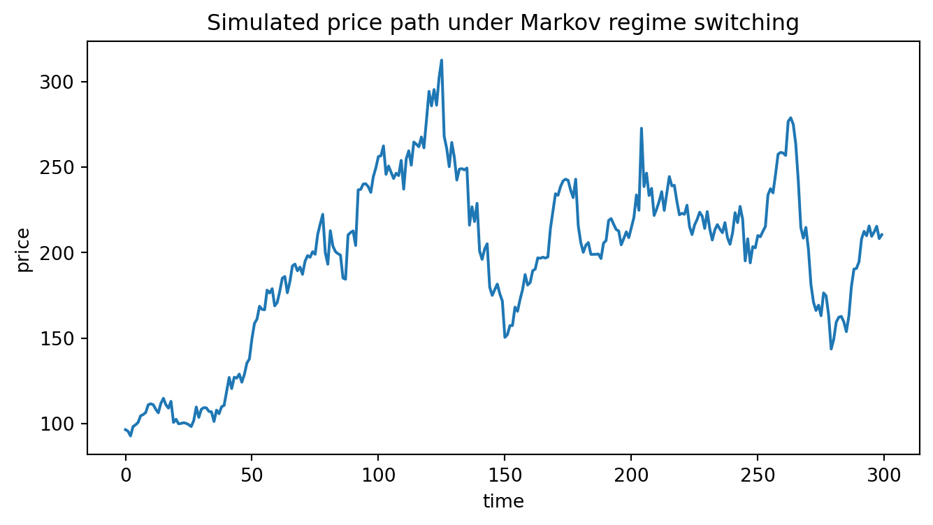
A Markov chain can be coupled with a return model. Let $X_t$ denote the market regime at time $t$. Conditional on $X_t=i$, suppose the next log return is
$$
r_{t+1}=\mu_i+\sigma_i\epsilon_{t+1},
\qquad
\epsilon_{t+1}\sim N(0,1).
$$
Here $\mu_i$ and $\sigma_i$ depend on the current regime. A simple bull--bear specification might be
$$
\mu_{\text{bear}}=-0.015,
\qquad
\sigma_{\text{bear}}=0.060,
$$
and
$$
\mu_{\text{bull}}=0.010,
\qquad
\sigma_{\text{bull}}=0.030.
$$
The unconditional return distribution is a mixture of regime-specific distributions. If the current regime distribution is $\alpha_t$, then
$$
\mathbb E[r_{t+1}\mid \mathcal F_t]
=
\sum_i \mathbb P(X_t=i\mid\mathcal F_t)\mu_i.
$$
The conditional variance is
$$
\operatorname{Var}(r_{t+1}\mid\mathcal F_t)
=
\sum_i p_i\sigma_i^2
+
\sum_i p_i(\mu_i-\bar\mu)^2,
$$
where $p_i=\mathbb P(X_t=i\mid\mathcal F_t)$ and $\bar\mu=\sum_i p_i\mu_i$. The first term is average within-regime variance. The second term is between-regime variance.
::: {.callout-note}
## Statistical interpretation
Regime switching creates non-normal unconditional returns even when conditional returns are normal inside each regime. This is one mathematical explanation for volatility clustering and heavy-tailed empirical return histograms.
:::
```{python}
#| label: ch09-simulate-regime-switching-returns
#| fig-cap: "Simulated regime-switching log returns."
rng = np.random.default_rng(7243)

P = np.array([
    [0.85, 0.15],  # bear row
    [0.08, 0.92]   # bull row
])
mu = np.array([-0.015, 0.010])
sigma = np.array([0.060, 0.030])
state_names = np.array(["bear", "bull"])

T = 300
states = np.zeros(T, dtype=int)
returns = np.zeros(T)
states[0] = 1  # start in bull

for t in range(1, T):
    states[t] = rng.choice([0, 1], p=P[states[t - 1]])

returns = rng.normal(mu[states], sigma[states])
prices = 100 * np.exp(np.cumsum(returns))

fig, ax = plt.subplots(figsize=(8, 4))
ax.plot(prices)
ax.set_title("Simulated price path under Markov regime switching")
ax.set_xlabel("time")
ax.set_ylabel("price")
plt.show()

pd.Series(state_names[states]).value_counts(normalize=True)
```
```{python}
#| label: ch09-return-mixture-summary
summary = pd.DataFrame({
    "regime": state_names,
    "mean_log_return": mu,
    "volatility": sigma,
    "stationary_probability": pi
})
summary
```
## 9.9 Interactive Demo: Regime Mixture and Tail Risk
In this demo, returns are modeled as a mixture of two normal distributions. The mixture weights are interpreted as current regime probabilities.
<div class="interactive-card">
<h3>Explore a two-regime return mixture</h3>
<p>The bull regime has a higher mean and lower volatility. The bear regime has a lower mean and higher volatility. Move the slider to change the probability of the bear regime.</p>
<div class="mf-controls">
<label for="mf-ch09-bear-weight">bear-regime probability</label>
<input id="mf-ch09-bear-weight" type="range" min="0.00" max="1.00" step="0.01" value="0.30">
<span id="mf-ch09-bear-weight-val">0.30</span>
</div>
<div id="mf-ch09-mixture-plot" class="plotly-demo"></div>
<div id="mf-ch09-mixture-output" class="mf-output"></div>
</div>
<script>
if (window.mfPlotlyReady) {
window.mfPlotlyReady(function() {
var slider = document.getElementById("mf-ch09-bear-weight");
var value = document.getElementById("mf-ch09-bear-weight-val");
var output = document.getElementById("mf-ch09-mixture-output");
var plot = document.getElementById("mf-ch09-mixture-plot");
if (!slider || !plot || typeof Plotly === "undefined") return;
function normalPdf(x, mu, sigma) {
var z = (x - mu) / sigma;
return Math.exp(-0.5 * z * z) / (sigma * Math.sqrt(2 * Math.PI));
}
function update() {
var wBear = Number(slider.value);
var wBull = 1 - wBear;
value.textContent = wBear.toFixed(2);
var muBear = -0.015;
var sigmaBear = 0.060;
var muBull = 0.010;
var sigmaBull = 0.030;
var x = [];
var yBear = [];
var yBull = [];
var yMix = [];
for (var k = 0; k <= 300; k++) {
var r = -0.18 + 0.0012 * k;
x.push(r);
var fb = normalPdf(r, muBear, sigmaBear);
var fu = normalPdf(r, muBull, sigmaBull);
yBear.push(wBear * fb);
yBull.push(wBull * fu);
yMix.push(wBear * fb + wBull * fu);
}
var mean = wBear * muBear + wBull * muBull;
var second = wBear * (sigmaBear * sigmaBear + muBear * muBear) + wBull * (sigmaBull * sigmaBull + muBull * muBull);
var variance = second - mean * mean;
Plotly.newPlot(plot, [
{x: x, y: yMix, mode: "lines", name: "mixture density"},
{x: x, y: yBear, mode: "lines", name: "weighted bear component", line: {dash: "dash"}},
{x: x, y: yBull, mode: "lines", name: "weighted bull component", line: {dash: "dot"}}
], {
title: "Two-Regime Return Mixture",
xaxis: {title: "one-period log return"},
yaxis: {title: "density"},
margin: {l: 55, r: 20, t: 50, b: 50}
}, {responsive: true});
output.innerHTML = "Mixture mean = " + mean.toFixed(4) + ", mixture volatility = " + Math.sqrt(variance).toFixed(4) + ".";
}
slider.addEventListener("input", update);
update();
});
}
</script>
The important lesson is that regime uncertainty contributes to risk in two ways. First, each regime has its own volatility. Second, uncertainty about the regime adds additional variance through different regime means.
## 9.10 Markov Rewards and Cumulative Returns
A Markov reward model assigns a reward $g(i)$ to each state $i$. In finance, the reward can represent expected return, cost, spread, default loss, or utility.
Let $g$ be a column vector with entries $g_i$. If the initial distribution is $\alpha_0$, then the expected one-period reward at time $t$ is
$$
\mathbb E[g(X_t)]=\alpha_0P^tg.
$$
The expected cumulative reward over periods $0,1,\ldots,T-1$ is
$$
\mathbb E\left[\sum_{t=0}^{T-1}g(X_t)\right]
=
\sum_{t=0}^{T-1}\alpha_0P^tg.
$$
With discount factor $\beta\in(0,1)$, the expected discounted reward is
$$
\mathbb E\left[\sum_{t=0}^{T-1}\beta^tg(X_t)\right]
=
\sum_{t=0}^{T-1}\beta^t\alpha_0P^tg.
$$
For an infinite horizon, if $\beta<1$,
$$
\sum_{t=0}^{\infty}\beta^tP^t=(I-\beta P)^{-1},
$$
so
$$
\mathbb E\left[\sum_{t=0}^{\infty}\beta^tg(X_t)\right]
=
\alpha_0(I-\beta P)^{-1}g.
$$
::: {.example}
### Example 9.3: Discounted expected return by regime
Suppose the expected monthly log return is $-1.5\%$ in bear and $1.0\%$ in bull. Let
$$
g=\begin{pmatrix}-0.015\\0.010\end{pmatrix}.
$$
If $\beta=0.99$ and $\alpha_0=(0,1)$, then the discounted expected cumulative return is
$$
\alpha_0(I-\beta P)^{-1}g.
$$
:::
```{python}
#| label: ch09-markov-reward
P = np.array([
    [0.85, 0.15],
    [0.08, 0.92]
])
g = np.array([-0.015, 0.010])
alpha0 = np.array([0.0, 1.0])
beta = 0.99

finite_horizon = sum((beta ** t) * (alpha0 @ np.linalg.matrix_power(P, t) @ g) for t in range(60))
infinite_horizon = alpha0 @ np.linalg.inv(np.eye(2) - beta * P) @ g

print("60-period discounted expected reward:", finite_horizon)
print("infinite-horizon discounted expected reward:", infinite_horizon)
```
## 9.11 Credit-Rating Transition Matrices
Markov chains are widely used in credit-risk modeling. A credit rating can be treated as a state. A simplified rating state space might be
$$
\mathcal S=\{A,B,D\},
$$
where $D$ denotes default. A transition matrix might be
$$
P=
\begin{pmatrix}
0.92 & 0.07 & 0.01\\
0.10 & 0.82 & 0.08\\
0.00 & 0.00 & 1.00
\end{pmatrix}.
$$
The default state is absorbing because
$$
P_{DD}=1.
$$
In this model, once default happens, the chain remains in default. The probability of default within $n$ periods starting from rating $i$ is
$$
\mathbb P_i(X_n=D)=(P^n)_{iD}.
$$
::: {.definition}
### Definition 9.6: Absorbing state
A state $i$ is absorbing if
$$
P_{ii}=1.
$$
Once an absorbing state is entered, it is never left.
:::
```{python}
#| label: ch09-credit-transition
P_credit = np.array([
    [0.92, 0.07, 0.01],
    [0.10, 0.82, 0.08],
    [0.00, 0.00, 1.00]
])
ratings = ["A", "B", "D"]

rows = []
for n in [1, 2, 5, 10]:
    Pn = np.linalg.matrix_power(P_credit, n)
    rows.append({
        "horizon": n,
        "default_prob_start_A": Pn[0, 2],
        "default_prob_start_B": Pn[1, 2]
    })

pd.DataFrame(rows)
```
The matrix-power calculation is easy, but the modeling assumptions are strong. A real credit model must address macroeconomic covariates, rating momentum, recovery rates, and risk-neutral versus physical transition probabilities.
## 9.12 Hitting Probabilities
A hitting time is the first time a chain enters a specified set. For credit risk, the set may be the default state. For risk management, it may be a crisis regime.
Let $A\subseteq\mathcal S$ and define
$$
\tau_A=\inf\{t\ge 0:X_t\in A\}.
$$
The probability of ever hitting $A$ from state $i$ is
$$
h_i=\mathbb P_i(\tau_A<\infty).
$$
The vector $h$ satisfies boundary conditions
$$
h_i=1 \quad \text{for } i\in A,
$$
and the harmonic equations
$$
h_i=\sum_jP_{ij}h_j
\quad \text{for } i\notin A.
$$
This is a system of linear equations.
::: {.example}
### Example 9.4: Probability of eventual default
In the three-state credit model above, default is absorbing and accessible from both non-default states. Therefore the eventual default probability is $1$ from both $A$ and $B$. In finite-horizon problems, however, the default probability is less than $1$ and is computed by $P^n$.
:::
## 9.13 Hidden Markov Models
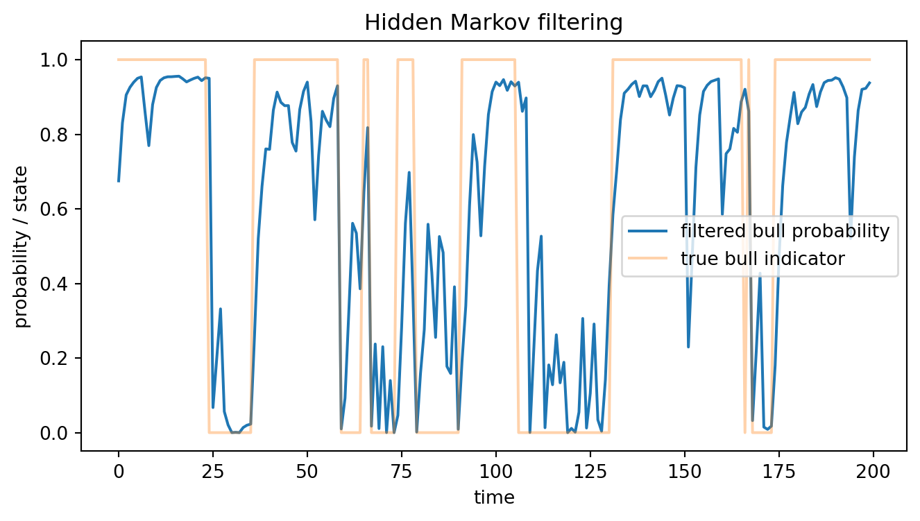
In many applications, the regime is not directly observed. We observe returns, spreads, or volatility proxies, but not the true state $X_t$. A hidden Markov model has two layers:
1. a hidden regime process $(X_t)$ that is a Markov chain;
2. observed data $(Y_t)$ whose distribution depends on the hidden state.
A simple model is
$$
X_t\sim \text{Markov}(P),
$$
and
$$
Y_t\mid X_t=i\sim N(\mu_i,\sigma_i^2).
$$
The filtering problem is to compute
$$
\mathbb P(X_t=i\mid Y_1,\ldots,Y_t).
$$
This is a conditional probability updated recursively as new observations arrive.
For a finite-state hidden Markov model, define the filtered probability row vector
$$
\phi_t(i)=\mathbb P(X_t=i\mid Y_1,
\ldots,Y_t).
$$
The update has two steps.
First, predict the next regime:
$$
\widehat\phi_t=\phi_{t-1}P.
$$
Second, update using the likelihood of the observation $Y_t$:
$$
\phi_t(i)
=
\frac{\widehat\phi_t(i) f_i(Y_t)}{\sum_j\widehat\phi_t(j) f_j(Y_t)},
$$
where $f_i$ is the density of $Y_t$ conditional on state $i$.
```{python}
#| label: ch09-hmm-filter
#| fig-cap: "Filtering hidden bull probability from simulated returns."
from math import sqrt, pi, exp

rng = np.random.default_rng(2026)
P = np.array([
    [0.90, 0.10],
    [0.07, 0.93]
])
mu = np.array([-0.020, 0.008])
sigma = np.array([0.055, 0.025])
T = 200

states = np.zeros(T, dtype=int)
y = np.zeros(T)
states[0] = 1
for t in range(1, T):
    states[t] = rng.choice([0, 1], p=P[states[t - 1]])
y = rng.normal(mu[states], sigma[states])

def normal_pdf(x, mean, sd):
    z = (x - mean) / sd
    return exp(-0.5 * z * z) / (sd * sqrt(2 * pi))

phi = np.array([0.5, 0.5])
filtered = []
for obs in y:
    pred = phi @ P
    likelihood = np.array([normal_pdf(obs, mu[i], sigma[i]) for i in range(2)])
    phi = pred * likelihood
    phi = phi / phi.sum()
    filtered.append(phi.copy())

filtered = np.array(filtered)

plt.figure(figsize=(8, 4))
plt.plot(filtered[:, 1], label="filtered bull probability")
plt.plot(states, alpha=0.35, label="true bull indicator")
plt.xlabel("time")
plt.ylabel("probability / state")
plt.title("Hidden Markov filtering")
plt.legend()
plt.show()
```
::: {.warning}
Hidden Markov models are useful but delicate. Regimes can be hard to identify, likelihoods may have multiple local optima, and fitted states do not automatically have economic meaning. A regime labeled as bull or bear is an interpretation, not a theorem.
:::
## 9.14 Markov Chains Under Physical and Pricing Measures
In earlier chapters, we distinguished the physical probability measure $\mathbb P$ from the risk-neutral measure $\mathbb Q$. The same distinction applies to Markov chains.
Under the physical measure, a transition matrix $P$ may describe real-world regime frequencies:
$$
P_{ij}=\mathbb P(X_{t+1}=j\mid X_t=i).
$$
Under a pricing measure, another transition matrix $Q$ may be used:
$$
Q_{ij}=\mathbb Q(X_{t+1}=j\mid X_t=i).
$$
The matrix $Q$ is not chosen merely to fit historical transitions. It must be consistent with no-arbitrage pricing of traded risks. For a Markovian payoff $H(X_T)$ and deterministic one-period risk-free gross return $R$, the risk-neutral price is
$$
V_t(i)=\frac{1}{R}\sum_j Q_{ij}V_{t+1}(j).
$$
In vector form,
$$
V_t=\frac{1}{R}QV_{t+1}.
$$
By iterating backward,
$$
V_0=R^{-T}Q^TH,
$$
where $H$ is treated as a column vector of terminal payoffs.
::: {.example}
### Example 9.5: Pricing a regime payoff
Suppose a derivative pays $1$ if the economy is in the bull state after $T$ periods and pays $0$ otherwise. If $H=(0,1)^\top$, then the price at state $i$ is
$$
V_0(i)=R^{-T}(Q^TH)_i.
$$
This is the discounted risk-neutral probability of ending in the bull state.
:::
```{python}
#| label: ch09-markov-pricing
Q = np.array([
    [0.82, 0.18],
    [0.12, 0.88]
])
R = 1.004
T = 12
H = np.array([0.0, 1.0])  # pays 1 in bull state at maturity

price_by_initial_state = (np.linalg.matrix_power(Q, T) @ H) / (R ** T)
print("price starting from bear:", price_by_initial_state[0])
print("price starting from bull:", price_by_initial_state[1])
```
This example is intentionally simple. In a full asset-pricing model, the pricing transition matrix $Q$ must be connected to traded assets, state prices, and the absence of arbitrage.
## 9.15 Estimating Transition Matrices
If regimes are observed, the maximum likelihood estimator for a transition matrix is simple. Let $N_{ij}$ be the number of observed transitions from state $i$ to state $j$. Then
$$
\widehat P_{ij}=\frac{N_{ij}}{\sum_k N_{ik}}.
$$
This estimator is just the empirical conditional frequency.
```{python}
#| label: ch09-estimate-transition-matrix
rng = np.random.default_rng(101)
P_true = np.array([
    [0.85, 0.15],
    [0.08, 0.92]
])
T = 1000
states = np.zeros(T, dtype=int)
states[0] = 1
for t in range(1, T):
    states[t] = rng.choice([0, 1], p=P_true[states[t - 1]])

counts = np.zeros((2, 2), dtype=int)
for t in range(T - 1):
    counts[states[t], states[t + 1]] += 1

P_hat = counts / counts.sum(axis=1, keepdims=True)
print("transition counts")
print(counts)
print("estimated transition matrix")
print(P_hat)
```
If regimes are hidden, transition estimation is harder. One commonly uses maximum likelihood with the forward algorithm or the expectation-maximization algorithm. The main statistical issues include sample size, local optima, and the danger of over-interpreting states.
## 9.16 Model Checking and Financial Interpretation
A Markov regime model should not be accepted just because it fits a dataset. Important checks include:
- Are the rows of the estimated transition matrix valid probabilities?
- Are the regimes persistent enough to be economically meaningful?
- Are the fitted regime means and volatilities stable across samples?
- Does the model improve out-of-sample forecasting or risk estimation?
- Are the regimes observable, hidden, or defined by an external rule?
- Is the matrix under the physical measure or a pricing measure?
::: {.callout-tip}
## Common modeling mistake
A high-volatility state is not automatically a crisis state. A statistically fitted state is a mathematical component of a model. Economic interpretation requires additional evidence.
:::
## 9.17 AI-Assisted Learning Components
AI tools can help with Markov-chain computations, but they often make convention errors. The most common mistakes are transposing the transition matrix, confusing $P^n$ with elementwise powers, and mixing physical and risk-neutral transition probabilities.
::: {.callout-tip}
## AI prompt: transition-matrix audit
Use the following prompt after writing a Markov-chain solution.
> I am using row probability vectors and a row-stochastic transition matrix $P$. Audit my Markov-chain calculation. Check whether each row of $P$ sums to one, whether I should compute $\alpha_0P^n$ or $P^n\alpha_0$, whether my stationary distribution satisfies $\pi P=\pi$, and whether I confused physical probabilities with pricing probabilities.
:::
::: {.callout-tip}
## AI prompt: regime-model explanation
> Explain this two-state regime-switching return model to an MS statistics student. Emphasize the difference between the hidden regime process, the conditional return distribution, and the unconditional mixture distribution. State the assumptions clearly and list three ways the model could fail empirically.
:::
::: {.callout-tip}
## AI prompt: code review
> Review this Python code for simulating a finite Markov chain. Check that `rng.choice` receives the correct row of the transition matrix, that the estimated transition matrix normalizes by rows, and that the stationary distribution is computed using the correct left eigenvector convention.
:::
## 9.18 Chapter Summary
This chapter introduced finite-state Markov chains as a mathematical language for regime dynamics. The key points are:
- a Markov chain satisfies the conditional independence condition that the future depends on the present state, not on the full past;
- a transition matrix $P$ is row-stochastic when its rows are probability distributions;
- with row-vector distributions, the update is $\alpha_{t+1}=\alpha_tP$;
- multi-step transition probabilities are entries of $P^n$;
- stationary distributions solve $\pi P=\pi$;
- irreducibility and aperiodicity imply convergence to the unique stationary distribution;
- Markov chains can model bull--bear regimes, credit-rating transitions, and hidden states;
- Markov reward models compute expected cumulative rewards through matrix sums;
- hidden Markov models update filtered regime probabilities using prediction and Bayes normalization;
- pricing applications require careful distinction between physical and risk-neutral transition matrices.
## Exercises
### Conceptual Exercises
1. Explain the Markov property in your own words. Give one financial example where it may be plausible and one where it may be too restrictive.
2. Suppose $P$ is row-stochastic. Why does each row sum to one? What financial interpretation does a row have in a regime model?
3. Explain the difference between the physical transition matrix $P$ and the pricing transition matrix $Q$.
4. Why can a mixture of normal distributions have heavier tails than a single normal distribution?
5. Explain why a hidden Markov regime should not automatically be interpreted as a bull or bear market.
### Computational Exercises
6. Let
$$
P=
\begin{pmatrix}
0.70 & 0.30\\
0.20 & 0.80
\end{pmatrix}.
$$
Compute $P^2$, $P^5$, and the stationary distribution.
7. For the matrix in Exercise 6, suppose $\alpha_0=(1,0)$. Compute $\alpha_0P^n$ for $n=1,2,5,10$.
8. Derive the stationary distribution formula for the two-state matrix
$$
P=
\begin{pmatrix}
1-a & a\\
b & 1-b
\end{pmatrix}.
$$
9. Suppose a credit-rating model has states $A,B,D$ and transition matrix
$$
P=
\begin{pmatrix}
0.94 & 0.05 & 0.01\\
0.08 & 0.84 & 0.08\\
0 & 0 & 1
\end{pmatrix}.
$$
Compute the three-year default probability starting from $A$ and starting from $B$.
10. Let $g=(-0.02,0.01)^\top$ and $\beta=0.98$. For a two-state chain with
$$
P=
\begin{pmatrix}
0.85 & 0.15\\
0.10 & 0.90
\end{pmatrix},
$$
compute $\alpha_0(I-\beta P)^{-1}g$ for $\alpha_0=(0,1)$.
### Proof Exercises
11. Prove the Chapman--Kolmogorov equation for $n$ steps by induction.
12. Prove that if $\pi$ is stationary, then $\pi P^n=\pi$ for every $n\ge 1$.
13. For a finite irreducible chain, explain why all states must have positive stationary probability.
14. Show that if $P$ is row-stochastic, then $P\mathbf 1=\mathbf 1$, where $\mathbf 1$ is the column vector of all ones.
15. For the two-state transition matrix above, show that the second eigenvalue is $1-a-b$.
### Python Exercises
16. Write a Python function `simulate_markov_chain(P, initial_state, T, rng)` that returns a simulated path.
17. Write a Python function `stationary_distribution(P)` that solves $\pi P=\pi$ and $\sum_i\pi_i=1$.
18. Simulate a three-state market model with states calm, volatile, and crisis. Assign different means and volatilities to the three states and plot the resulting price path.
19. Estimate a transition matrix from a simulated state sequence and compare it with the true matrix.
20. Implement the hidden Markov filtering recursion for a two-state Gaussian observation model.
### AI-Assisted Exercises
21. Ask an AI tool to explain why $\alpha_0P^n$ is the correct formula under the row-vector convention. Then identify whether the explanation distinguishes row and column conventions clearly.
22. Give an AI tool an intentionally invalid transition matrix whose rows do not sum to one. Ask it to find and fix the problem.
23. Ask an AI tool to compare a regime-switching normal model with a GARCH model. Write a short critique of the response.
24. Use an AI tool to review your Python code for estimating a transition matrix. Check whether it correctly catches row-normalization errors.
25. Ask an AI tool to explain the difference between observed regimes and hidden regimes. Rewrite the answer in precise mathematical language.