---
title: "Chapter 20. Short-Rate Models"
---
::: {.chapter-objectives}
## Learning Goals
By the end of this chapter, students should be able to:
- define the short rate and explain its connection to the money-market account;
- derive the risk-neutral bond-pricing formula for zero-coupon bonds;
- state and use the bond-pricing PDE for one-factor short-rate models;
- simulate Vasicek and CIR short-rate dynamics;
- derive the affine bond-price form $P(t,T)=A(t,T)e^{-B(t,T)r_t}$;
- compute Vasicek and CIR zero-coupon bond prices and continuously compounded yields;
- explain mean reversion, volatility, negative rates, and the Feller condition;
- distinguish physical-measure estimation from risk-neutral pricing;
- use Python to simulate short-rate models, price bonds, and audit numerical results;
- use AI tools carefully to check formulas, assumptions, and implementation details.
:::
::: {.hero-box}
In equity modeling, the basic risky state variable is often the stock price $S_t$. In fixed income, the central state variable is often the **short rate** $r_t$, the instantaneous interest rate over a very small time interval.
The guiding pricing formula of this chapter is
$$
P(t,T)
=
\mathbb E^{\mathbb Q}\left[
\exp\left(-\int_t^T r_s\,ds\right)
\middle|\mathcal F_t
\right],
$$
where $P(t,T)$ is the time-$t$ price of a zero-coupon bond paying $1$ at maturity $T$.
This formula says: to price a riskless future payoff in a stochastic interest-rate world, discount by the entire future path of the short rate and take expectation under the risk-neutral measure.
:::
## 20.1 Why Short-Rate Models?
Chapter 19 treated the yield curve as an object observed at one date. We learned how to price deterministic cash flows once the discount curve $T\mapsto P(t,T)$ is given.
This chapter asks a deeper modeling question:
> How should the discount curve evolve randomly through time?
A **short-rate model** answers this question by modeling the instantaneous rate $r_t$. Once the short-rate process is specified under a pricing measure, zero-coupon bond prices are obtained by discounting along future short-rate paths.
The short rate is not directly the same as a one-year yield or a ten-year yield. Instead, it is the infinitesimal rate that drives the money-market account.
::: {.definition}
## Short rate
The short rate $r_t$ is the instantaneous continuously compounded interest rate at time $t$. Informally,
$$
r_t
\approx
\text{the annualized interest rate from } t \text{ to } t+dt.
$$
The associated money-market account satisfies
$$
dB_t=r_tB_t\,dt,
\qquad B_0=1.
$$
:::
Solving this ordinary differential equation gives
$$
B_t = \exp\left(\int_0^t r_s\,ds\right).
$$
Therefore the stochastic discount factor from time $t$ to time $T$ generated by the short-rate path is
$$
\frac{B_t}{B_T}
=
\exp\left(-\int_t^T r_s\,ds\right).
$$
This is the mathematical reason why integrals of $r_s$ appear in fixed-income pricing.
## 20.2 The Money-Market Account and Discounting
Suppose $r_t$ is known over the interval $[0,T]$. Then a riskless investment of one dollar grows to
$$
B_T = \exp\left(\int_0^T r_s\,ds\right).
$$
Equivalently, one dollar paid at time $T$ has time-$0$ value
$$
\exp\left(-\int_0^T r_s\,ds\right)
$$
if the entire short-rate path is known in advance.
In reality, the future path of $r_s$ is random. Therefore the time-$t$ value of a future deterministic payoff must average over future interest-rate paths under a pricing measure.
::: {.theorem}
## Risk-neutral zero-coupon bond pricing
Let $B_t=\exp(\int_0^t r_s\,ds)$ be the money-market account. Under an equivalent martingale measure $\mathbb Q$, the time-$t$ price of a zero-coupon bond paying $1$ at time $T$ is
$$
P(t,T)
=
B_t\mathbb E^{\mathbb Q}\left[\frac{1}{B_T}\middle|\mathcal F_t\right]
=
\mathbb E^{\mathbb Q}\left[
\exp\left(-\int_t^T r_s\,ds\right)
\middle|\mathcal F_t
\right].
$$
:::
### Proof idea
Under $\mathbb Q$, every discounted traded asset price should be a martingale. The zero-coupon bond pays $P(T,T)=1$. Hence its discounted value satisfies
$$
\frac{P(t,T)}{B_t}
=
\mathbb E^{\mathbb Q}\left[\frac{P(T,T)}{B_T}\middle|\mathcal F_t\right]
=
\mathbb E^{\mathbb Q}\left[\frac{1}{B_T}\middle|\mathcal F_t\right].
$$
Multiplying by $B_t$ gives the formula.
::: {.callout-important}
## Pricing measure, not forecasting measure
The expectation in the bond-pricing formula is under $\mathbb Q$, not necessarily under the real-world measure $\mathbb P$. The drift of the short-rate process used for pricing may be different from the drift estimated from historical data.
:::
## 20.3 One-Factor Short-Rate Models
A one-factor short-rate model assumes that all randomness in the term structure is driven by one Brownian motion and one state variable $r_t$.
Under the risk-neutral measure $\mathbb Q$, a common model has the form
$$
dr_t = \alpha(t,r_t)\,dt + \beta(t,r_t)\,dW_t^{\mathbb Q}.
$$
Here:
- $\alpha(t,r)$ is the risk-neutral drift;
- $\beta(t,r)$ is the short-rate volatility;
- $W_t^{\mathbb Q}$ is Brownian motion under the pricing measure;
- $r_t$ is the state variable that summarizes the information relevant for bond pricing.
If the model is Markovian, then the bond price can be written as a deterministic function of time and the current short rate:
$$
P(t,T)=p(t,r_t;T).
$$
The maturity $T$ is fixed, while $t$ and $r$ are variables.
## 20.4 The Bond-Pricing PDE
The risk-neutral expectation formula implies a partial differential equation. This is a direct application of the Feynman--Kac principle.
::: {.theorem}
## Bond-pricing PDE
Assume that under $\mathbb Q$,
$$
dr_t = \alpha(t,r_t)\,dt + \beta(t,r_t)\,dW_t^{\mathbb Q}.
$$
If the zero-coupon bond price has the form
$$
P(t,T)=p(t,r_t;T),
$$
then $p$ satisfies
$$
p_t(t,r;T)
+\alpha(t,r)p_r(t,r;T)
+\frac12\beta^2(t,r)p_{rr}(t,r;T)
-rp(t,r;T)
=0,
$$
with terminal condition
$$
p(T,r;T)=1.
$$
:::
### Interpretation of each term
The term $p_t$ measures calendar-time decay. The term $\alpha p_r$ accounts for the risk-neutral mean movement of the short rate. The term $\frac12\beta^2p_{rr}$ is the convexity correction from short-rate volatility. The term $-rp$ discounts the future payoff at the current short rate.
::: {.remark}
## Why the PDE differs from the Black--Scholes PDE
In the Black--Scholes PDE, the stock is traded and its risk premium is eliminated by delta hedging. In a short-rate model, the short rate itself is not generally a traded asset. The risk adjustment is already embedded in the risk-neutral drift $\alpha$.
:::
## 20.5 Affine Term-Structure Models
Many important short-rate models have **affine** bond prices:
$$
P(t,T)=A(t,T)e^{-B(t,T)r_t}.
$$
Equivalently,
$$
\log P(t,T)=\log A(t,T)-B(t,T)r_t.
$$
This means that the log bond price is an affine function of the current short rate.
::: {.definition}
## Affine short-rate model
A one-factor short-rate model is called affine if its zero-coupon bond prices can be written as
$$
P(t,T)=\exp\{C(t,T)-B(t,T)r_t\},
$$
where $B(t,T)$ and $C(t,T)$ are deterministic functions.
:::
The affine form is powerful because it converts a PDE problem into ordinary differential equations for $B$ and $C$.
In the models below, we write $\tau=T-t$ for time to maturity and express bond prices as
$$
P(t,T)=A(\tau)e^{-B(\tau)r_t}.
$$
## 20.6 The Vasicek Model
The Vasicek model assumes that the short rate follows an Ornstein--Uhlenbeck process under $\mathbb Q$:
$$
dr_t = a(b-r_t)\,dt + \sigma\,dW_t^{\mathbb Q},
\qquad a>0,
\quad \sigma>0.
$$
The parameters have clear interpretations:
- $a$ is the speed of mean reversion;
- $b$ is the long-run mean under the pricing measure;
- $\sigma$ is the instantaneous volatility of the short rate.
The drift pulls the rate toward $b$. If $r_t>b$, then $a(b-r_t)<0$ and the rate tends to move downward. If $r_t<b$, then $a(b-r_t)>0$ and the rate tends to move upward.
::: {.callout-note}
## Mean reversion
Mean reversion is essential in many interest-rate models. It says that very high rates tend to fall and very low rates tend to rise, at least on average under the chosen measure.
:::
### Explicit solution
The Vasicek model is a linear SDE. Its solution is
$$
r_t
=
b+(r_0-b)e^{-at}
+\sigma\int_0^t e^{-a(t-s)}\,dW_s^{\mathbb Q}.
$$
Therefore $r_t$ is normally distributed with mean
$$
\mathbb E^{\mathbb Q}[r_t]
=
b+(r_0-b)e^{-at},
$$
and variance
$$
\operatorname{Var}^{\mathbb Q}(r_t)
=
\frac{\sigma^2}{2a}\left(1-e^{-2at}\right).
$$
As $t\to\infty$,
$$
r_t \Rightarrow N\left(b,\frac{\sigma^2}{2a}\right).
$$
### Negative-rate limitation
Because the Vasicek short rate is Gaussian, it can become negative with positive probability. This is not necessarily a mathematical error; negative rates have appeared in real markets. But if the modeling goal requires strictly nonnegative rates, Vasicek may be inappropriate.
## 20.7 Vasicek Zero-Coupon Bond Prices
Under the risk-neutral Vasicek model,
$$
dr_t = a(b-r_t)\,dt + \sigma\,dW_t^{\mathbb Q},
$$
the zero-coupon bond price is affine:
$$
P(t,T)=A(\tau)e^{-B(\tau)r_t},
\qquad \tau=T-t.
$$
The functions are
$$
B(\tau)=\frac{1-e^{-a\tau}}{a},
$$
and
$$
A(\tau)
=
\exp\left\{
\left(b-\frac{\sigma^2}{2a^2}\right)(B(\tau)-\tau)
-
\frac{\sigma^2}{4a}B(\tau)^2
\right\}.
$$
Thus
$$
P(t,T)
=
\exp\left\{
\left(b-\frac{\sigma^2}{2a^2}\right)(B(\tau)-\tau)
-
\frac{\sigma^2}{4a}B(\tau)^2
-B(\tau)r_t
\right\}.
$$
The continuously compounded yield is
$$
R(t,T)=-\frac{\log P(t,T)}{T-t}.
$$
::: {.example}
## Vasicek bond price
Suppose
$$
r_t=0.04,\quad a=0.6,\quad b=0.05,\quad \sigma=0.015,\quad T-t=5.
$$
Then
$$
B(5)=\frac{1-e^{-3}}{0.6}\approx 1.5837.
$$
After computing $A(5)$, the five-year zero-coupon bond price is
$$
P(t,T)=A(5)e^{-1.5837 r_t}.
$$
This formula shows directly how the current short rate affects the whole yield curve.
:::
## 20.8 Interactive Demo: Vasicek and CIR Short-Rate Paths
The following interactive example compares simulated paths of Vasicek and CIR short rates. The two models can have similar mean-reversion behavior, but their treatment of volatility near zero is different.
::: {.interactive-card}
### Simulated short-rate paths
<div class="mf-control-row">
<label for="ch20-path-model">Model</label>
<select id="ch20-path-model">
<option value="vasicek">Vasicek</option>
<option value="cir">CIR</option>
</select>
<span class="mf-badge" id="ch20-path-model-value">Vasicek</span>
</div>
<div class="mf-control-row">
<label for="ch20-r0">Initial rate $r_0$</label>
<input id="ch20-r0" type="range" min="0" max="10" step="0.25" value="4">
<span class="mf-badge" id="ch20-r0-value">4.00%</span>
</div>
<div class="mf-control-row">
<label for="ch20-a">Mean-reversion speed $a$</label>
<input id="ch20-a" type="range" min="5" max="200" step="5" value="60">
<span class="mf-badge" id="ch20-a-value">0.60</span>
</div>
<div class="mf-control-row">
<label for="ch20-b">Long-run mean $b$</label>
<input id="ch20-b" type="range" min="0" max="10" step="0.25" value="5">
<span class="mf-badge" id="ch20-b-value">5.00%</span>
</div>
<div class="mf-control-row">
<label for="ch20-sigma">Volatility $\sigma$</label>
<input id="ch20-sigma" type="range" min="1" max="20" step="1" value="3">
<span class="mf-badge" id="ch20-sigma-value">3.00%</span>
</div>
<div id="ch20-short-rate-paths" class="plotly-demo"></div>
<div id="ch20-short-rate-paths-note" class="mf-output"></div>
:::
<script>
window.mfPlotlyReady(function() {
var plotId = "ch20-short-rate-paths";
var noteId = "ch20-short-rate-paths-note";
var modelInput = document.getElementById("ch20-path-model");
var r0Input = document.getElementById("ch20-r0");
var aInput = document.getElementById("ch20-a");
var bInput = document.getElementById("ch20-b");
var sigmaInput = document.getElementById("ch20-sigma");
var modelValue = document.getElementById("ch20-path-model-value");
var r0Value = document.getElementById("ch20-r0-value");
var aValue = document.getElementById("ch20-a-value");
var bValue = document.getElementById("ch20-b-value");
var sigmaValue = document.getElementById("ch20-sigma-value");
function seededNormalFactory(seed) {
var state = seed >>> 0;
function uniform() {
state = (1664525 * state + 1013904223) >>> 0;
return (state + 1) / 4294967297;
}
return function() {
var u1 = Math.max(uniform(), 1e-12);
var u2 = uniform();
return Math.sqrt(-2 * Math.log(u1)) * Math.cos(2 * Math.PI * u2);
};
}
function simulatePath(model, r0, a, b, sigma, T, n, seed) {
var dt = T / n;
var z = seededNormalFactory(seed);
var x = [0];
var y = [r0];
var r = r0;
for (var i = 1; i <= n; i++) {
if (model === "vasicek") {
r = r + a * (b - r) * dt + sigma * Math.sqrt(dt) * z();
} else {
r = r + a * (b - r) * dt + sigma * Math.sqrt(Math.max(r, 0)) * Math.sqrt(dt) * z();
r = Math.max(r, 0);
}
x.push(i * dt);
y.push(r);
}
return {x: x, y: y};
}
function update() {
var model = modelInput.value;
var r0 = Number(r0Input.value) / 100;
var a = Number(aInput.value) / 100;
var b = Number(bInput.value) / 100;
var sigma = Number(sigmaInput.value) / 100;
var T = 10;
var n = 500;
var traces = [];
for (var k = 0; k < 8; k++) {
var path = simulatePath(model, r0, a, b, sigma, T, n, 7000 + 97 * k);
traces.push({
x: path.x,
y: path.y.map(function(v) { return 100 * v; }),
mode: "lines",
name: "path " + (k + 1),
line: {width: 1.5}
});
}
var title = model === "vasicek" ? "Vasicek Short-Rate Paths" : "CIR Short-Rate Paths";
Plotly.newPlot(plotId, traces, {
title: title,
xaxis: {title: "time in years"},
yaxis: {title: "short rate (%)"},
margin: {l: 60, r: 20, t: 55, b: 50}
}, {responsive: true});
modelValue.textContent = model === "vasicek" ? "Vasicek" : "CIR";
r0Value.textContent = (100 * r0).toFixed(2) + "%";
aValue.textContent = a.toFixed(2);
bValue.textContent = (100 * b).toFixed(2) + "%";
sigmaValue.textContent = (100 * sigma).toFixed(2) + "%";
var note = model === "vasicek"
? "Vasicek rates are Gaussian. They mean-revert, but negative simulated rates are possible."
: "CIR volatility is proportional to the square root of the rate. With full truncation, simulated rates remain nonnegative.";
document.getElementById(noteId).textContent = note;
}
[modelInput, r0Input, aInput, bInput, sigmaInput].forEach(function(el) {
el.addEventListener("input", update);
el.addEventListener("change", update);
});
update();
});
</script>
## 20.9 The CIR Model
The Cox--Ingersoll--Ross model modifies the Vasicek model by making volatility proportional to $\sqrt{r_t}$:
$$
dr_t = a(b-r_t)\,dt + \sigma\sqrt{r_t}\,dW_t^{\mathbb Q},
\qquad a>0,
\quad b>0,
\quad \sigma>0.
$$
The parameters again represent mean reversion speed, long-run level, and volatility. The key difference is that the diffusion coefficient becomes small near zero.
This square-root structure helps keep the process nonnegative.
::: {.theorem}
## Feller condition
For the CIR model
$$
dr_t = a(b-r_t)\,dt + \sigma\sqrt{r_t}\,dW_t,
$$
if
$$
2ab\ge \sigma^2,
$$
then the boundary $0$ is unattainable from positive initial values. If $2ab<\sigma^2$, the process can reach zero, but it remains nonnegative in the continuous-time model.
:::
The CIR model is widely used because interest rates and intensity-like quantities are often naturally nonnegative.
### Conditional distribution
The CIR transition distribution is related to a noncentral chi-square distribution. For this course, the most important points are:
- the model is mean-reverting;
- the diffusion coefficient is state-dependent;
- exact simulation is possible but more technical than Vasicek;
- Euler simulation should be handled carefully near zero.
A common numerical method is the **full truncation Euler scheme**:
$$
r_{n+1}
=
r_n+a(b-r_n^+)\Delta t
+\sigma\sqrt{r_n^+}\sqrt{\Delta t}Z_{n+1},
\qquad r_n^+=\max(r_n,0),
$$
followed by truncation if needed.
## 20.10 CIR Zero-Coupon Bond Prices
Under the risk-neutral CIR model,
$$
dr_t = a(b-r_t)\,dt + \sigma\sqrt{r_t}\,dW_t^{\mathbb Q},
$$
zero-coupon bond prices also have the affine form
$$
P(t,T)=A(\tau)e^{-B(\tau)r_t},
\qquad \tau=T-t.
$$
Define
$$
\gamma = \sqrt{a^2+2\sigma^2}.
$$
Then
$$
B(\tau)
=
\frac{2(e^{\gamma\tau}-1)}{(\gamma+a)(e^{\gamma\tau}-1)+2\gamma},
$$
and
$$
A(\tau)
=
\left[
\frac{2\gamma e^{(a+\gamma)\tau/2}}
{(\gamma+a)(e^{\gamma\tau}-1)+2\gamma}
\right]^{2ab/\sigma^2}.
$$
Therefore,
$$
P(t,T)=A(\tau)e^{-B(\tau)r_t}.
$$
The continuously compounded yield is again
$$
R(t,T)=-\frac{\log P(t,T)}{\tau}.
$$
::: {.callout-warning}
## Parameter interpretation depends on the measure
In the formulas above, $a$, $b$, and $\sigma$ are risk-neutral parameters. If parameters are estimated from historical short-rate data under $\mathbb P$, a market-price-of-risk adjustment is usually needed before using them for pricing.
:::
## 20.11 Interactive Demo: Bond Prices and Yield Curves
This interactive demo compares Vasicek and CIR zero-coupon bond prices and continuously compounded yields. Both models generate affine bond prices, but their volatility structures produce different yield-curve behavior.
::: {.interactive-card}
### Affine bond prices from short-rate models
<div class="mf-control-row">
<label for="ch20-curve-model">Model</label>
<select id="ch20-curve-model">
<option value="vasicek">Vasicek</option>
<option value="cir">CIR</option>
</select>
<span class="mf-badge" id="ch20-curve-model-value">Vasicek</span>
</div>
<div class="mf-control-row">
<label for="ch20-curve-r0">Current short rate $r_t$</label>
<input id="ch20-curve-r0" type="range" min="0" max="10" step="0.25" value="4">
<span class="mf-badge" id="ch20-curve-r0-value">4.00%</span>
</div>
<div class="mf-control-row">
<label for="ch20-curve-a">Mean-reversion speed $a$</label>
<input id="ch20-curve-a" type="range" min="5" max="200" step="5" value="60">
<span class="mf-badge" id="ch20-curve-a-value">0.60</span>
</div>
<div class="mf-control-row">
<label for="ch20-curve-b">Long-run mean $b$</label>
<input id="ch20-curve-b" type="range" min="0" max="10" step="0.25" value="5">
<span class="mf-badge" id="ch20-curve-b-value">5.00%</span>
</div>
<div class="mf-control-row">
<label for="ch20-curve-sigma">Volatility $\sigma$</label>
<input id="ch20-curve-sigma" type="range" min="1" max="20" step="1" value="3">
<span class="mf-badge" id="ch20-curve-sigma-value">3.00%</span>
</div>
<div id="ch20-bond-curve" class="plotly-demo"></div>
<div id="ch20-bond-curve-note" class="mf-output"></div>
:::
<script>
window.mfPlotlyReady(function() {
var modelInput = document.getElementById("ch20-curve-model");
var r0Input = document.getElementById("ch20-curve-r0");
var aInput = document.getElementById("ch20-curve-a");
var bInput = document.getElementById("ch20-curve-b");
var sigmaInput = document.getElementById("ch20-curve-sigma");
var modelValue = document.getElementById("ch20-curve-model-value");
var r0Value = document.getElementById("ch20-curve-r0-value");
var aValue = document.getElementById("ch20-curve-a-value");
var bValue = document.getElementById("ch20-curve-b-value");
var sigmaValue = document.getElementById("ch20-curve-sigma-value");
function vasicekPrice(tau, r, a, b, sigma) {
if (tau <= 0) return 1;
var B = (1 - Math.exp(-a * tau)) / a;
var logA = (b - sigma * sigma / (2 * a * a)) * (B - tau) - (sigma * sigma * B * B) / (4 * a);
return Math.exp(logA - B * r);
}
function cirPrice(tau, r, a, b, sigma) {
if (tau <= 0) return 1;
var gamma = Math.sqrt(a * a + 2 * sigma * sigma);
var eg = Math.exp(gamma * tau);
var denom = (gamma + a) * (eg - 1) + 2 * gamma;
var B = 2 * (eg - 1) / denom;
var A = Math.pow(2 * gamma * Math.exp((a + gamma) * tau / 2) / denom, 2 * a * b / (sigma * sigma));
return A * Math.exp(-B * r);
}
function update() {
var model = modelInput.value;
var r = Number(r0Input.value) / 100;
var a = Number(aInput.value) / 100;
var b = Number(bInput.value) / 100;
var sigma = Number(sigmaInput.value) / 100;
var taus = [];
var prices = [];
var yields = [];
for (var i = 1; i <= 120; i++) {
var tau = i / 6;
var p = model === "vasicek"
? vasicekPrice(tau, r, a, b, sigma)
: cirPrice(tau, r, a, b, sigma);
taus.push(tau);
prices.push(p);
yields.push(-100 * Math.log(p) / tau);
}
var traces = [
{
x: taus,
y: prices,
mode: "lines",
name: "zero-coupon price",
yaxis: "y"
},
{
x: taus,
y: yields,
mode: "lines",
name: "zero yield (%)",
yaxis: "y2"
}
];
Plotly.newPlot("ch20-bond-curve", traces, {
title: (model === "vasicek" ? "Vasicek" : "CIR") + " Bond Prices and Zero Yields",
xaxis: {title: "maturity in years"},
yaxis: {title: "price P(0,T)", range: [0, 1.15]},
yaxis2: {title: "zero yield (%)", overlaying: "y", side: "right"},
legend: {orientation: "h", y: -0.25},
margin: {l: 60, r: 65, t: 55, b: 80}
}, {responsive: true});
modelValue.textContent = model === "vasicek" ? "Vasicek" : "CIR";
r0Value.textContent = (100 * r).toFixed(2) + "%";
aValue.textContent = a.toFixed(2);
bValue.textContent = (100 * b).toFixed(2) + "%";
sigmaValue.textContent = (100 * sigma).toFixed(2) + "%";
var feller = 2 * a * b - sigma * sigma;
var note = model === "cir"
? "CIR Feller value 2ab - sigma^2 = " + feller.toFixed(5) + ". Nonnegative rates are structurally built into the model."
: "Vasicek gives closed-form Gaussian rates, which can be analytically convenient but may allow negative rates.";
document.getElementById("ch20-bond-curve-note").textContent = note;
}
[modelInput, r0Input, aInput, bInput, sigmaInput].forEach(function(el) {
el.addEventListener("input", update);
el.addEventListener("change", update);
});
update();
});
</script>
## 20.12 Physical Drift Versus Risk-Neutral Drift
Historical estimation is usually performed under the physical probability measure $\mathbb P$. Pricing requires a risk-neutral measure $\mathbb Q$.
Suppose under $\mathbb P$ the Vasicek model is
$$
dr_t=\kappa(\theta-r_t)\,dt+\sigma\,dW_t^{\mathbb P}.
$$
If the market price of short-rate risk is a constant $\lambda$, and
$$
dW_t^{\mathbb Q}=dW_t^{\mathbb P}+\lambda\,dt,
$$
then
$$
dW_t^{\mathbb P}=dW_t^{\mathbb Q}-\lambda\,dt.
$$
Substituting gives
$$
dr_t
=
\left[\kappa(\theta-r_t)-\sigma\lambda\right]dt
+\sigma\,dW_t^{\mathbb Q}.
$$
This can be written as
$$
dr_t=\kappa(\theta^{\mathbb Q}-r_t)\,dt+\sigma\,dW_t^{\mathbb Q},
$$
where
$$
\theta^{\mathbb Q}=\theta-\frac{\sigma\lambda}{\kappa}.
$$
Thus the long-run mean used for pricing may differ from the long-run mean estimated from historical data.
::: {.callout-important}
## Estimation is not calibration
Estimating a model from historical rates gives physical-measure parameters. Calibrating to bond prices, swaps, caps, floors, or swaptions gives risk-neutral parameters or risk-neutral curves. These are related, but they are not the same problem.
:::
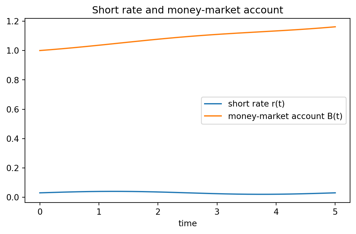
## 20.13 Python Example: Money-Market Account from a Short-Rate Path
```{python}
import numpy as np
import pandas as pd
import matplotlib.pyplot as plt

# A deterministic time-varying short-rate curve for illustration.
T = 5.0
n = 501
t = np.linspace(0, T, n)
r = 0.03 + 0.01 * np.sin(2 * np.pi * t / T)

dt = t[1] - t[0]
integral_r = np.cumsum(r) * dt
B = np.exp(integral_r)
discount = 1 / B

summary = pd.DataFrame({
    "time": t[::100],
    "short_rate": r[::100],
    "money_market_account": B[::100],
    "discount_factor": discount[::100]
})
summary
```
```{python}
plt.figure(figsize=(7, 4))
plt.plot(t, r, label="short rate r(t)")
plt.plot(t, B, label="money-market account B(t)")
plt.xlabel("time")
plt.title("Short rate and money-market account")
plt.legend()
plt.show()
```
The key point is that $B_t$ depends on the accumulated short-rate integral, not only on the current value $r_t$.
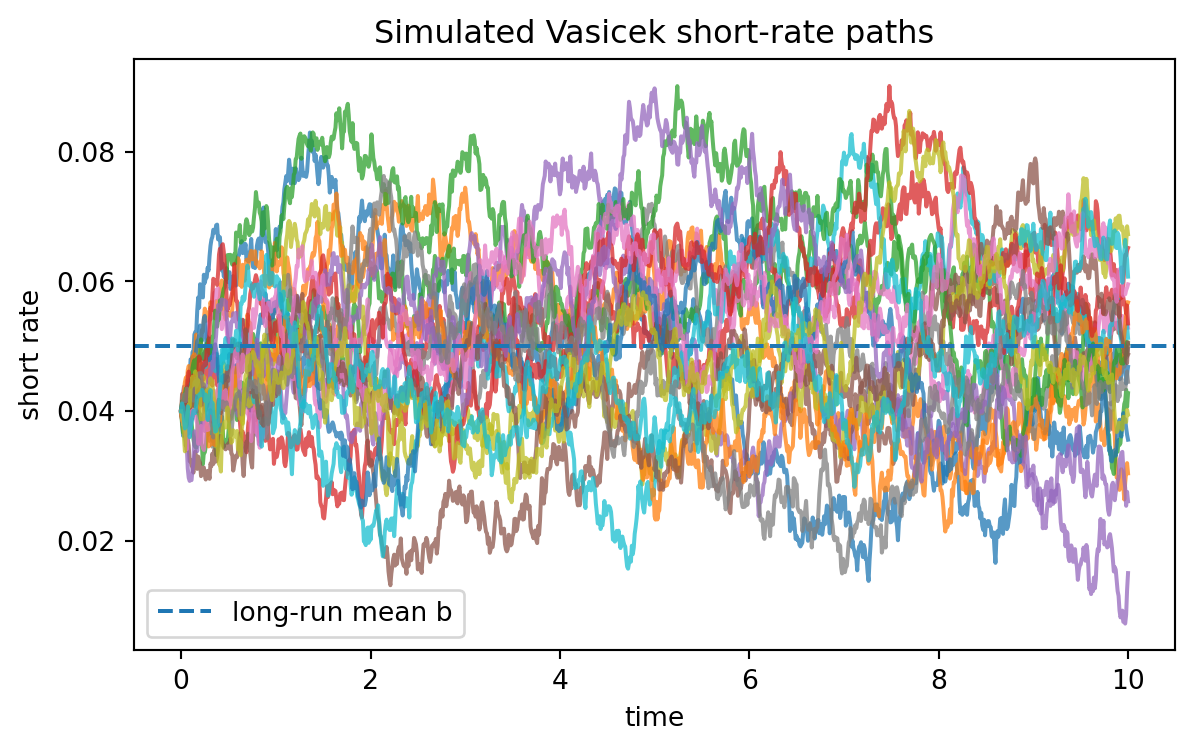
## 20.14 Python Example: Simulating Vasicek Paths
```{python}
import numpy as np
import matplotlib.pyplot as plt

rng = np.random.default_rng(7243)

def simulate_vasicek(r0=0.04, a=0.6, b=0.05, sigma=0.015, T=10, n_steps=1000, n_paths=20):
    dt = T / n_steps
    rates = np.empty((n_paths, n_steps + 1))
    rates[:, 0] = r0
    for k in range(n_steps):
        z = rng.normal(size=n_paths)
        rates[:, k + 1] = rates[:, k] + a * (b - rates[:, k]) * dt + sigma * np.sqrt(dt) * z
    times = np.linspace(0, T, n_steps + 1)
    return times, rates

times, vasicek_paths = simulate_vasicek()

plt.figure(figsize=(7, 4))
plt.plot(times, vasicek_paths.T, alpha=0.75)
plt.axhline(0.05, linestyle="--", label="long-run mean b")
plt.xlabel("time")
plt.ylabel("short rate")
plt.title("Simulated Vasicek short-rate paths")
plt.legend()
plt.show()
```
The paths fluctuate randomly but tend to move back toward the long-run mean $b$.
### Check the conditional mean and variance
```{python}
r0 = 0.04
a = 0.6
b = 0.05
sigma = 0.015
T = 3
n_steps = 600
n_paths = 20000

times, paths = simulate_vasicek(r0, a, b, sigma, T, n_steps, n_paths)
terminal = paths[:, -1]

theory_mean = b + (r0 - b) * np.exp(-a * T)
theory_var = sigma**2 / (2 * a) * (1 - np.exp(-2 * a * T))

print("Empirical mean:", terminal.mean())
print("Theory mean:   ", theory_mean)
print("Empirical var: ", terminal.var(ddof=1))
print("Theory var:    ", theory_var)
```
This is a useful model-audit step: if the simulation is correct, empirical moments should be close to the theoretical moments when the number of paths is large.
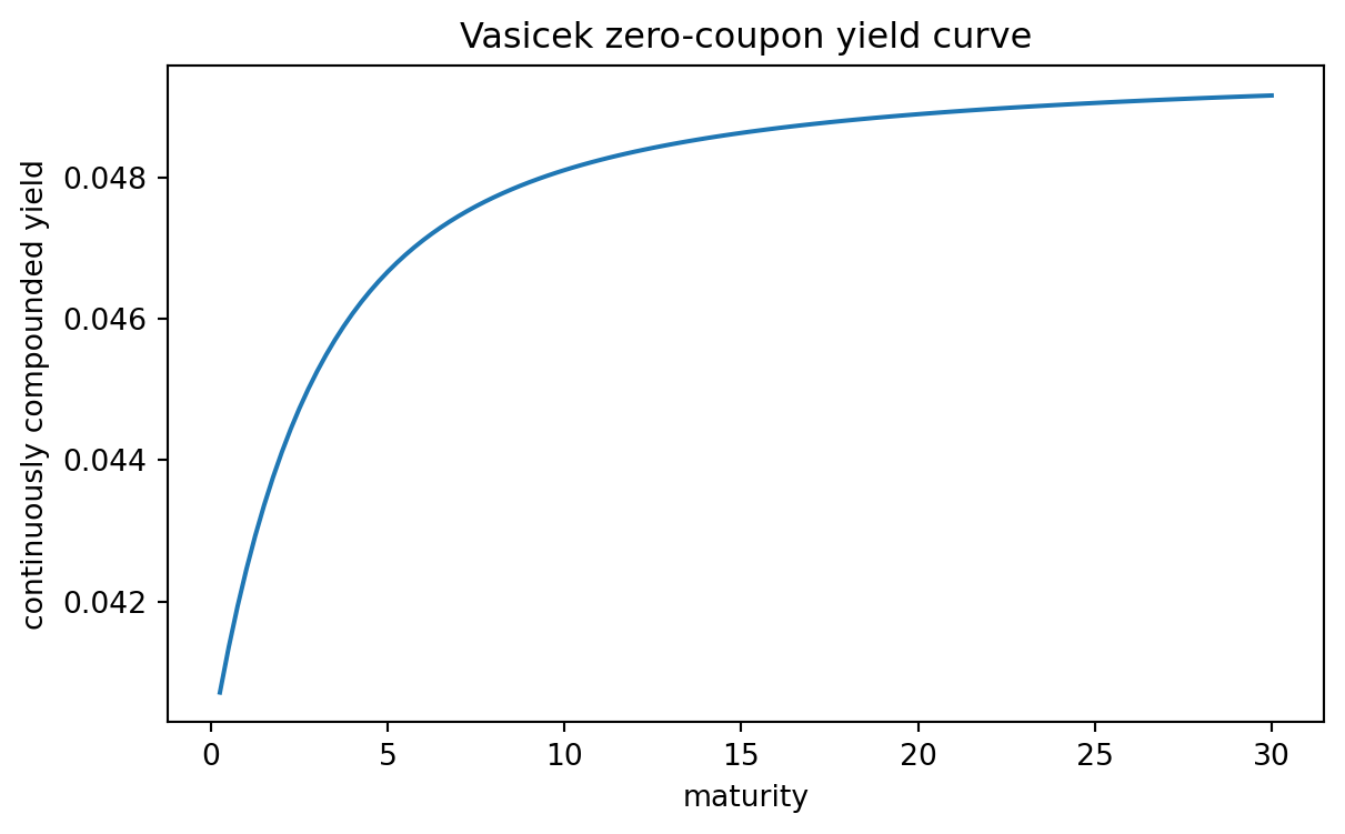
## 20.15 Python Example: Vasicek Bond Prices and Yields
```{python}
def vasicek_B(tau, a):
    return (1 - np.exp(-a * tau)) / a

def vasicek_A(tau, a, b, sigma):
    B = vasicek_B(tau, a)
    log_A = (b - sigma**2 / (2 * a**2)) * (B - tau) - (sigma**2 * B**2) / (4 * a)
    return np.exp(log_A)

def vasicek_bond_price(r, tau, a=0.6, b=0.05, sigma=0.015):
    B = vasicek_B(tau, a)
    A = vasicek_A(tau, a, b, sigma)
    return A * np.exp(-B * r)

r_current = 0.04
maturities = np.linspace(0.25, 30, 120)
prices = vasicek_bond_price(r_current, maturities)
yields = -np.log(prices) / maturities

pd.DataFrame({
    "maturity": maturities[::20],
    "price": prices[::20],
    "zero_yield": yields[::20]
})
```
```{python}
plt.figure(figsize=(7, 4))
plt.plot(maturities, yields)
plt.xlabel("maturity")
plt.ylabel("continuously compounded yield")
plt.title("Vasicek zero-coupon yield curve")
plt.show()
```
## 20.16 Python Example: Monte Carlo Check of Vasicek Bond Pricing
The analytic formula should agree with Monte Carlo pricing under $\mathbb Q$:
$$
P(0,T)=\mathbb E^{\mathbb Q}\left[\exp\left(-\int_0^T r_s\,ds\right)\right].
$$
```{python}
def mc_vasicek_bond_price(r0=0.04, a=0.6, b=0.05, sigma=0.015, T=5, n_steps=1000, n_paths=50000, seed=11):
    rng_local = np.random.default_rng(seed)
    dt = T / n_steps
    r = np.full(n_paths, r0)
    integral = np.zeros(n_paths)
    for _ in range(n_steps):
        integral += r * dt
        z = rng_local.normal(size=n_paths)
        r = r + a * (b - r) * dt + sigma * np.sqrt(dt) * z
    discounts = np.exp(-integral)
    return discounts.mean(), discounts.std(ddof=1) / np.sqrt(n_paths)

mc_price, mc_se = mc_vasicek_bond_price()
closed_form = vasicek_bond_price(0.04, 5.0)

print("Monte Carlo price:", mc_price)
print("Monte Carlo SE:   ", mc_se)
print("Closed-form price:", closed_form)
print("Difference:       ", mc_price - closed_form)
```
The Monte Carlo estimator has simulation error. The closed-form formula is the benchmark.
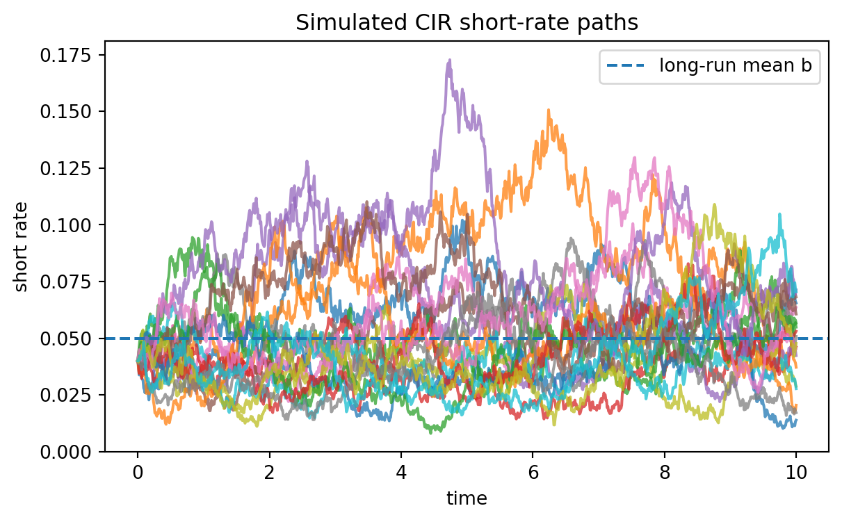
## 20.17 Python Example: Simulating CIR Paths
```{python}
def simulate_cir(r0=0.04, a=0.6, b=0.05, sigma=0.10, T=10, n_steps=1000, n_paths=20, seed=123):
    rng_local = np.random.default_rng(seed)
    dt = T / n_steps
    rates = np.empty((n_paths, n_steps + 1))
    rates[:, 0] = r0
    for k in range(n_steps):
        r_plus = np.maximum(rates[:, k], 0)
        z = rng_local.normal(size=n_paths)
        next_r = rates[:, k] + a * (b - r_plus) * dt + sigma * np.sqrt(r_plus) * np.sqrt(dt) * z
        rates[:, k + 1] = np.maximum(next_r, 0)
    times = np.linspace(0, T, n_steps + 1)
    return times, rates

times, cir_paths = simulate_cir()

plt.figure(figsize=(7, 4))
plt.plot(times, cir_paths.T, alpha=0.75)
plt.axhline(0.05, linestyle="--", label="long-run mean b")
plt.xlabel("time")
plt.ylabel("short rate")
plt.title("Simulated CIR short-rate paths")
plt.legend()
plt.show()

print("Minimum simulated rate:", cir_paths.min())
```
Because the diffusion coefficient is $\sigma\sqrt{r_t}$, volatility becomes smaller when the short rate is close to zero.
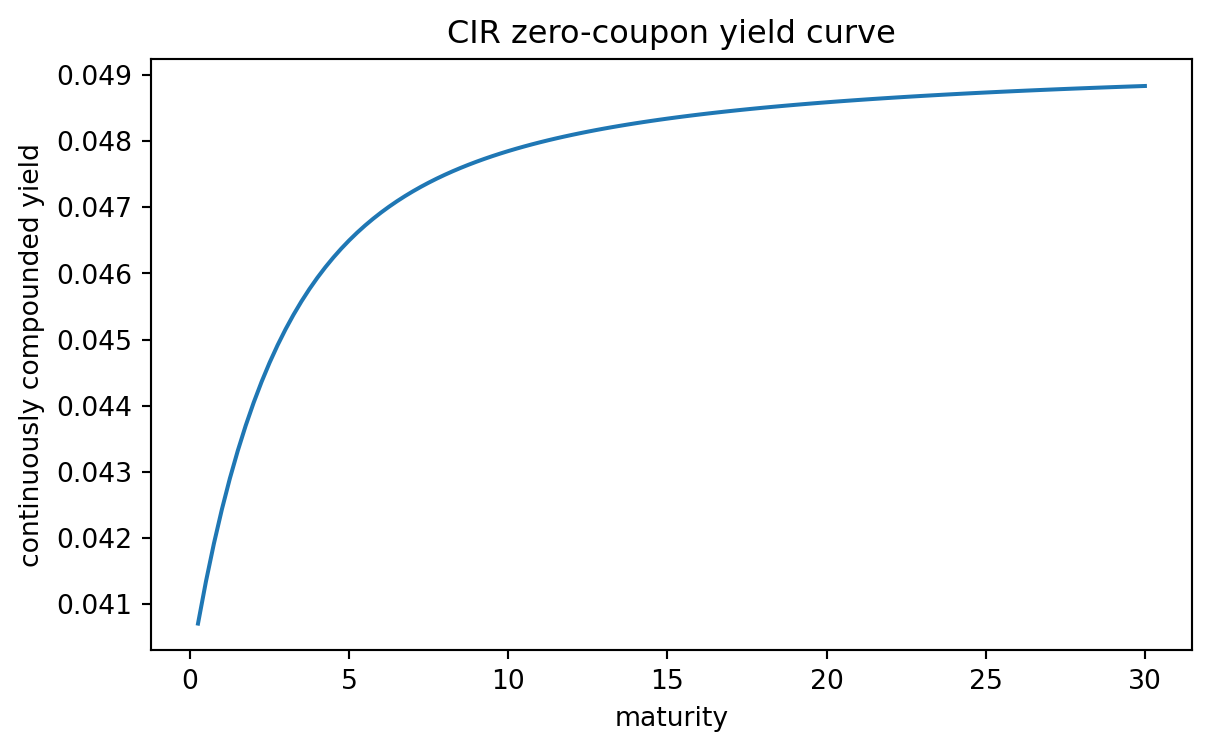
## 20.18 Python Example: CIR Bond Prices and the Feller Condition
```{python}
def cir_B(tau, a, sigma):
    gamma = np.sqrt(a**2 + 2 * sigma**2)
    exp_gt = np.exp(gamma * tau)
    return 2 * (exp_gt - 1) / ((gamma + a) * (exp_gt - 1) + 2 * gamma)

def cir_A(tau, a, b, sigma):
    gamma = np.sqrt(a**2 + 2 * sigma**2)
    exp_gt = np.exp(gamma * tau)
    denom = (gamma + a) * (exp_gt - 1) + 2 * gamma
    base = 2 * gamma * np.exp((a + gamma) * tau / 2) / denom
    return base ** (2 * a * b / sigma**2)

def cir_bond_price(r, tau, a=0.6, b=0.05, sigma=0.10):
    return cir_A(tau, a, b, sigma) * np.exp(-cir_B(tau, a, sigma) * r)

a = 0.6
b = 0.05
sigma = 0.10
print("Feller value 2ab - sigma^2:", 2 * a * b - sigma**2)

maturities = np.linspace(0.25, 30, 120)
prices_cir = cir_bond_price(0.04, maturities, a, b, sigma)
yields_cir = -np.log(prices_cir) / maturities

plt.figure(figsize=(7, 4))
plt.plot(maturities, yields_cir)
plt.xlabel("maturity")
plt.ylabel("continuously compounded yield")
plt.title("CIR zero-coupon yield curve")
plt.show()
```
The Feller value is a quick diagnostic. If $2ab-\sigma^2$ is positive, the zero boundary is unattainable in the exact continuous-time model.
## 20.19 Python Example: Estimating a Vasicek Model by Regression
For discretely observed short rates, the exact Vasicek transition has the form
$$
r_{t+\Delta}
=
b(1-e^{-a\Delta})+e^{-a\Delta}r_t+\varepsilon_{t+\Delta}.
$$
This suggests an autoregressive regression
$$
r_{k+1}=c+\phi r_k+\varepsilon_{k+1}.
$$
Then
$$
a=-\frac{\log\phi}{\Delta},
\qquad
b=\frac{c}{1-\phi}.
$$
```{python}
# Simulate daily observations from Vasicek and estimate by OLS.
rng = np.random.default_rng(2026)
r0 = 0.04
a_true = 0.8
b_true = 0.05
sigma_true = 0.012
Delta = 1 / 252
n_obs = 2520

r = np.empty(n_obs + 1)
r[0] = r0
for k in range(n_obs):
    # exact transition moments
    phi = np.exp(-a_true * Delta)
    mean = b_true + (r[k] - b_true) * phi
    var = sigma_true**2 / (2 * a_true) * (1 - np.exp(-2 * a_true * Delta))
    r[k + 1] = mean + np.sqrt(var) * rng.normal()

x = r[:-1]
y = r[1:]
X = np.column_stack([np.ones_like(x), x])
c_hat, phi_hat = np.linalg.lstsq(X, y, rcond=None)[0]

a_hat = -np.log(phi_hat) / Delta
b_hat = c_hat / (1 - phi_hat)
residuals = y - X @ np.array([c_hat, phi_hat])
var_eps_hat = residuals.var(ddof=2)
sigma_hat = np.sqrt(var_eps_hat * 2 * a_hat / (1 - np.exp(-2 * a_hat * Delta)))

print("a true / estimated:", a_true, a_hat)
print("b true / estimated:", b_true, b_hat)
print("sigma true / estimated:", sigma_true, sigma_hat)
```
This estimates physical-measure parameters if the data are historical observations. Pricing may require calibration to market instruments instead.
## 20.20 Comparing Vasicek and CIR
| Feature | Vasicek | CIR |
|---|---:|---:|
| SDE | $dr_t=a(b-r_t)dt+\sigma dW_t$ | $dr_t=a(b-r_t)dt+\sigma\sqrt{r_t}dW_t$ |
| Distribution | Gaussian | Noncentral chi-square type |
| Negative rates | Possible | Nonnegative in continuous time |
| Volatility | Constant | State-dependent |
| Bond price | Affine | Affine |
| Analytical convenience | Very high | High |
| Natural for strictly positive rates | Less suitable | More suitable |
The best model depends on the application. For teaching stochastic calculus and affine pricing, Vasicek is exceptionally transparent. For nonnegative rates and intensity-like variables, CIR is more natural.
## 20.21 Common Mistakes
### Mistake 1: Using historical drift directly for pricing
Historical mean reversion describes real-world behavior under $\mathbb P$. Bond pricing requires risk-neutral dynamics under $\mathbb Q$.
### Mistake 2: Forgetting the integral of the short rate
The stochastic discount factor is
$$
\exp\left(-\int_t^T r_s\,ds\right),
$$
not simply $e^{-r_t(T-t)}$ unless the short rate is constant.
### Mistake 3: Treating the short rate as the full yield curve
A one-factor short-rate model says the entire yield curve is driven by $r_t$. This is a modeling assumption, not a market identity.
### Mistake 4: Simulating CIR with a naive Euler scheme
The naive Euler step can produce negative rates. Use exact simulation when available or a positivity-preserving approximation such as full truncation.
### Mistake 5: Ignoring numerical stability
Affine formulas can involve exponentials and powers. For long maturities or extreme parameters, compute log prices when possible.
## 20.22 AI-Assisted Learning Components
::: {.ai-box}
## AI prompt: explain the short-rate pricing formula
Ask an AI tool:
> Explain why the zero-coupon bond price in a short-rate model is
> $P(t,T)=\mathbb E^{\mathbb Q}[\exp(-\int_t^T r_s ds)\mid\mathcal F_t]$.
> Emphasize the role of the money-market account and the risk-neutral measure.
Then check whether the answer clearly distinguishes $\mathbb P$ from $\mathbb Q$.
:::
::: {.ai-box}
## AI prompt: formula audit for Vasicek and CIR
Ask an AI tool to verify the formulas for $A(\tau)$ and $B(\tau)$ in the Vasicek and CIR models. Then compare its answer against this chapter.
A good audit should check:
1. the sign in the exponent $e^{-B(\tau)r_t}$;
2. the definition of $\tau=T-t$;
3. the terminal condition $P(T,T)=1$;
4. the difference between $A(\tau)$ and $\log A(\tau)$;
5. the measure under which parameters are defined.
:::
::: {.ai-box}
## AI prompt: code review for short-rate simulation
Give an AI tool your simulation code and ask:
> Does this simulation accidentally use physical-measure parameters for pricing? Does the CIR simulation preserve nonnegative rates? Does the Monte Carlo estimator discount by the integral of the short rate rather than by the terminal short rate?
Use the response as a checklist, not as an authority.
:::
## 20.23 Exercises
### Conceptual exercises
1. Explain why the short rate is not the same object as a ten-year yield.
2. Why does the money-market account satisfy $B_t=\exp(\int_0^t r_s ds)$?
3. In the bond-pricing formula, why is the expectation taken under $\mathbb Q$ rather than $\mathbb P$?
4. Explain the financial meaning of mean reversion in a short-rate model.
5. Give one advantage and one limitation of the Vasicek model.
6. Give one advantage and one limitation of the CIR model.
### Mathematical exercises
1. Let $r_t$ be deterministic. Show that the risk-neutral pricing formula reduces to
$$
P(t,T)=\exp\left(-\int_t^T r_s\,ds\right).
$$
2. Starting from $dB_t=r_tB_tdt$, solve for $B_t$.
3. For the Vasicek model, derive
$$
\mathbb E[r_t]=b+(r_0-b)e^{-at}.
$$
4. For the Vasicek model, derive
$$
\operatorname{Var}(r_t)=\frac{\sigma^2}{2a}(1-e^{-2at}).
$$
5. Verify that $B(0)=0$ and $A(0)=1$ in the Vasicek bond-price formula.
6. Verify that $B(0)=0$ and $A(0)=1$ in the CIR bond-price formula.
7. Use the bond-pricing PDE to check the affine ansatz $P(t,T)=A(\tau)e^{-B(\tau)r}$ for Vasicek.
### Computational exercises
1. Simulate Vasicek paths for several values of $a$. Describe how mean-reversion speed changes the paths.
2. Simulate Vasicek paths for several values of $\sigma$. Estimate the probability that rates become negative.
3. Simulate CIR paths using both naive Euler and full truncation Euler. Compare the minimum simulated rates.
4. Plot Vasicek yield curves for different current short rates $r_t$.
5. Plot CIR yield curves for different volatility values $\sigma$.
6. Use Monte Carlo simulation to estimate a Vasicek zero-coupon bond price and compare with the affine formula.
7. Estimate Vasicek parameters from simulated data using OLS. Repeat for different sample sizes.
### AI-assisted exercises
1. Ask an AI tool to explain the Feller condition. Identify whether it correctly distinguishes "unattainable zero" from "nonnegative process."
2. Ask an AI tool to derive the Vasicek bond-price formula. Check whether it confuses $A(\tau)$ and $\log A(\tau)$.
3. Ask an AI tool to write CIR simulation code. Audit whether the code can produce negative rates.
4. Ask an AI tool to explain the difference between estimation and calibration in interest-rate modeling. Improve the answer using examples from this chapter.
## 20.24 Chapter Summary
This chapter introduced short-rate models, which describe the random evolution of instantaneous interest rates. The core pricing formula is
$$
P(t,T)
=
\mathbb E^{\mathbb Q}\left[
\exp\left(-\int_t^T r_s\,ds\right)
\middle|\mathcal F_t
\right].
$$
For Markovian one-factor models, this expectation satisfies the bond-pricing PDE
$$
p_t+\alpha p_r+\frac12\beta^2p_{rr}-rp=0,
\qquad p(T,r;T)=1.
$$
The Vasicek model gives Gaussian mean-reverting rates and closed-form affine bond prices. The CIR model gives nonnegative square-root rates and also has affine bond prices. Both models illustrate the central mathematical structure of fixed-income modeling: stochastic calculus, risk-neutral discounting, affine functions, PDEs, and careful distinction between physical and pricing measures.