---
title: "Chapter 21. Heath--Jarrow--Morton Framework"
---
::: {.chapter-objectives}
## Learning Goals
By the end of this chapter, students should be able to:
- define zero-coupon bond prices, spot rates, and instantaneous forward rates;
- recover a discount curve from a forward-rate curve and recover a forward curve from bond prices;
- explain why the HJM framework models the entire forward-rate curve instead of only the short rate;
- write the HJM forward-rate dynamics under the risk-neutral measure;
- derive and interpret the HJM no-arbitrage drift restriction;
- compute the drift restriction for common volatility specifications;
- understand the infinite-dimensional viewpoint and the Musiela parametrization;
- simulate a discretized one-factor HJM model in Python;
- connect HJM modeling with calibration, PCA, and modern data-driven term-structure modeling;
- use AI tools to audit sign conventions, no-arbitrage restrictions, and numerical simulations.
:::
::: {.hero-box}
Short-rate models start with one state variable $r_t$ and derive bond prices from it. The Heath--Jarrow--Morton framework reverses the viewpoint: it starts with the whole **forward-rate curve**
$$
T \mapsto f(t,T),
$$
and imposes exactly the drift condition needed to avoid arbitrage.
For a zero-coupon bond price $P(t,T)$, the forward curve is defined by
$$
P(t,T)=\exp\left(-\int_t^T f(t,u)\,du\right).
$$
The central HJM result says that under the risk-neutral measure, once the forward-rate volatility is specified, the forward-rate drift is no longer free. In the one-factor case,
$$
\alpha(t,T)
=
\sigma(t,T)\int_t^T \sigma(t,u)\,du.
$$
This is one of the cleanest examples of a mathematical finance principle: **no-arbitrage determines drift from volatility**.
:::
## 21.1 From Short Rates to the Whole Curve
Chapter 20 modeled the short rate $r_t$ directly. That approach is natural because the money-market account satisfies
$$
dB_t=r_tB_t\,dt.
$$
However, fixed-income markets trade instruments across many maturities. A one-month rate, a two-year rate, and a thirty-year rate can move differently. A single short rate does not directly describe the whole curve.
At a fixed time $t$, the zero-coupon bond price curve
$$
T \mapsto P(t,T), \qquad T\ge t,
$$
contains the market prices of default-free payments of one dollar at all future maturities. The HJM framework models the stochastic evolution of this whole curve through the instantaneous forward rate.
::: {.definition}
## Zero-coupon bond price
For $T\ge t$, $P(t,T)$ denotes the time-$t$ price of a default-free zero-coupon bond that pays $1$ at time $T$.
The boundary condition is
$$
P(T,T)=1.
$$
:::
A discount curve $T\mapsto P(t,T)$ is economically meaningful when it is positive and normally decreasing in maturity. If the discount curve is differentiable in $T$, we define the instantaneous forward rate as follows.
::: {.definition}
## Instantaneous forward rate
The instantaneous forward rate for maturity $T$ observed at time $t$ is
$$
f(t,T)
=
-\frac{\partial}{\partial T}\log P(t,T).
$$
:::
Integrating this identity from $t$ to $T$ gives
$$
\log P(t,T)-\log P(t,t)
=
-\int_t^T f(t,u)\,du.
$$
Since $P(t,t)=1$, we obtain the fundamental relation
$$
P(t,T)=\exp\left(-\int_t^T f(t,u)\,du\right).
$$
The short rate is the forward rate at the shortest maturity:
$$
r_t=f(t,t).
$$
This identity connects HJM to the short-rate models from Chapter 20.
## 21.2 Spot Rates, Forward Rates, and Discount Factors
The continuously compounded spot rate $y(t,T)$ is defined by
$$
P(t,T)=e^{-y(t,T)(T-t)}.
$$
Therefore,
$$
y(t,T)= -\frac{1}{T-t}\log P(t,T)
=\frac{1}{T-t}\int_t^T f(t,u)\,du.
$$
So the spot rate is an average of instantaneous forward rates over the interval $[t,T]$.
::: {.remark}
## Forward rates contain more local information than spot rates
The spot rate $y(t,T)$ averages the entire forward curve from $t$ to $T$. The instantaneous forward rate $f(t,T)$ describes the local slope of the discount curve near maturity $T$.
In continuous time, the forward curve is often the mathematically cleaner object because the bond price can be recovered by integration.
:::
::: {.example}
## A simple deterministic forward curve
Suppose at time $0$ the forward curve is
$$
f(0,T)=a+bT,
\qquad T\ge 0.
$$
Then
$$
P(0,T)
=
\exp\left(-\int_0^T (a+bu)\,du\right)
=
\exp\left(-aT-\frac12 bT^2\right).
$$
The continuously compounded spot rate is
$$
y(0,T)
= -\frac{1}{T}\log P(0,T)
= a+\frac12 bT.
$$
Thus a linear forward curve produces a linear spot curve with half the slope.
:::
## 21.3 Interactive: Forward Curve, Discount Curve, and Yield Curve
The following interactive example shows how one forward-rate curve generates both a discount curve and a spot-rate curve.
::: {.interactive-card}
### Forward curve to bond prices
Use the sliders to change the level, slope, and curvature of the initial forward curve
$$
f(0,T)=\ell+sT+c(T-5)^2.
$$
<div class="mf-control-row">
<label for="ch21-level">level $\ell$</label>
<input id="ch21-level" type="range" min="0.005" max="0.08" step="0.001" value="0.03">
<span id="ch21-level-value" class="mf-badge">0.030</span>
</div>
<div class="mf-control-row">
<label for="ch21-slope">slope $s$</label>
<input id="ch21-slope" type="range" min="-0.008" max="0.012" step="0.0005" value="0.002">
<span id="ch21-slope-value" class="mf-badge">0.0020</span>
</div>
<div class="mf-control-row">
<label for="ch21-curv">curvature $c$</label>
<input id="ch21-curv" type="range" min="-0.0015" max="0.0015" step="0.0001" value="0.0002">
<span id="ch21-curv-value" class="mf-badge">0.0002</span>
</div>
<div id="ch21-forward-curve-demo" class="plotly-demo"></div>
<script>
(function() {
function values() {
return {
level: Number(document.getElementById("ch21-level").value),
slope: Number(document.getElementById("ch21-slope").value),
curv: Number(document.getElementById("ch21-curv").value)
};
}
function forward(T, p) {
return Math.max(0.0001, p.level + p.slope * T + p.curv * Math.pow(T - 5, 2));
}
function cumulativeIntegral(T, p) {
var n = 400;
var h = T / n;
var sum = 0.5 * forward(0, p) + 0.5 * forward(T, p);
for (var i = 1; i < n; i++) sum += forward(i * h, p);
return h * sum;
}
function draw() {
var p = values();
document.getElementById("ch21-level-value").textContent = p.level.toFixed(3);
document.getElementById("ch21-slope-value").textContent = p.slope.toFixed(4);
document.getElementById("ch21-curv-value").textContent = p.curv.toFixed(4);
var T = [];
for (var i = 1; i <= 160; i++) T.push(i * 10 / 160);
var f = T.map(function(x) { return 100 * forward(x, p); });
var P = T.map(function(x) { return Math.exp(-cumulativeIntegral(x, p)); });
var y = T.map(function(x) { return 100 * cumulativeIntegral(x, p) / x; });
var traces = [
{x: T, y: f, mode: "lines", name: "forward rate f(0,T) (%)", yaxis: "y1"},
{x: T, y: y, mode: "lines", name: "spot yield y(0,T) (%)", yaxis: "y1"},
{x: T, y: P, mode: "lines", name: "discount P(0,T)", yaxis: "y2"}
];
var layout = {
title: "Forward rates, spot yields, and discount factors",
xaxis: {title: "maturity T"},
yaxis: {title: "rate (%)"},
yaxis2: {title: "discount factor", overlaying: "y", side: "right", range: [0, 1.05]},
legend: {orientation: "h"},
margin: {l: 55, r: 60, t: 55, b: 45}
};
Plotly.newPlot("ch21-forward-curve-demo", traces, layout, {responsive: true});
}
if (window.mfPlotlyReady) {
window.mfPlotlyReady(function() {
["ch21-level", "ch21-slope", "ch21-curv"].forEach(function(id) {
document.getElementById(id).addEventListener("input", draw);
});
draw();
});
}
})();
</script>
:::
## 21.4 The HJM State Variable
In a short-rate model, the state variable might be a scalar $r_t$. In the HJM framework, the state variable is the entire function
$$
T\mapsto f(t,T),
\qquad T\ge t.
$$
This is an infinite-dimensional state variable. At each time $t$, the model must describe how every maturity point $T$ changes.
A one-factor HJM model under a probability measure takes the form
$$
df(t,T)=\alpha(t,T)\,dt+\sigma(t,T)\,dW_t,
\qquad 0\le t\le T.
$$
Here:
- $f(t,T)$ is the instantaneous forward rate at time $t$ for maturity $T$;
- $\alpha(t,T)$ is the forward-rate drift;
- $\sigma(t,T)$ is the forward-rate volatility;
- the same Brownian increment $dW_t$ drives all maturity points in the one-factor model.
A $d$-factor model is
$$
df(t,T)
=
\alpha(t,T)\,dt+
\sum_{k=1}^d \sigma_k(t,T)\,dW_t^{(k)},
$$
where $W=(W^{(1)},\ldots,W^{(d)})$ is a $d$-dimensional Brownian motion.
The HJM idea is not simply to choose $\alpha$ and $\sigma$ arbitrarily. Under the risk-neutral measure, the drift $\alpha$ must be linked to the volatility functions $\sigma_k$.
## 21.5 Bond Price Dynamics from Forward-Rate Dynamics
To derive the HJM drift restriction, fix a maturity $T$ and define
$$
A(t,T)=\int_t^T f(t,u)\,du.
$$
Then
$$
P(t,T)=e^{-A(t,T)}.
$$
Assume a one-factor risk-neutral candidate model
$$
df(t,u)=\alpha(t,u)\,dt+\sigma(t,u)\,dW_t.
$$
Using the Leibniz rule,
$$
dA(t,T)
=
\left[-f(t,t)+\int_t^T \alpha(t,u)\,du\right]dt
+
\left[\int_t^T \sigma(t,u)\,du\right]dW_t.
$$
Since $f(t,t)=r_t$, define
$$
\Sigma(t,T)=\int_t^T \sigma(t,u)\,du.
$$
Then
$$
dA(t,T)
=
\left[-r_t+\int_t^T \alpha(t,u)\,du\right]dt
+
\Sigma(t,T)dW_t.
$$
Now apply Itô's formula to $P(t,T)=e^{-A(t,T)}$:
$$
\frac{dP(t,T)}{P(t,T)}
=
-dA(t,T)+\frac12(dA(t,T))^2.
$$
Because $(dA)^2=\Sigma(t,T)^2dt$, we obtain
$$
\frac{dP(t,T)}{P(t,T)}
=
\left[
r_t
-\int_t^T \alpha(t,u)\,du
+\frac12\Sigma(t,T)^2
\right]dt
-
\Sigma(t,T)dW_t.
$$
Under the risk-neutral measure $\mathbb Q$, every discounted traded asset price must be a martingale. Therefore the drift of every zero-coupon bond must be $r_t$:
$$
\frac{dP(t,T)}{P(t,T)}
=
r_t\,dt+\text{volatility term}.
$$
Thus the extra drift term must vanish:
$$
-\int_t^T \alpha(t,u)\,du
+�rac12\left(\int_t^T \sigma(t,u)\,du\right)^2=0.
$$
Equivalently,
$$
\int_t^T \alpha(t,u)\,du
=
\frac12\left(\int_t^T \sigma(t,u)\,du\right)^2.
$$
Differentiating both sides with respect to $T$ gives the HJM drift restriction.
::: {.theorem}
## One-factor HJM drift restriction
Under the risk-neutral measure $\mathbb Q$, suppose
$$
df(t,T)=\alpha(t,T)\,dt+\sigma(t,T)\,dW_t.
$$
If zero-coupon bonds are traded and the discounted bond prices are $\mathbb Q$-martingales, then the forward-rate drift must satisfy
$$
\alpha(t,T)
=
\sigma(t,T)\int_t^T \sigma(t,u)\,du.
$$
:::
This formula is the core mathematical result of the chapter.
## 21.6 Multi-Factor HJM Drift Restriction
In a multi-factor HJM model,
$$
df(t,T)=\alpha(t,T)\,dt+
\sum_{k=1}^d \sigma_k(t,T)\,dW_t^{(k)}.
$$
Define the integrated volatility vector
$$
\Sigma_k(t,T)=\int_t^T \sigma_k(t,u)\,du,
\qquad k=1,\ldots,d.
$$
Then the bond volatility vector is
$$
-\Sigma(t,T)=-(\Sigma_1(t,T),\ldots,\Sigma_d(t,T)).
$$
The HJM drift restriction becomes
$$
\alpha(t,T)
=
\sum_{k=1}^d \sigma_k(t,T)
\int_t^T \sigma_k(t,u)\,du.
$$
Equivalently, using vector notation,
$$
\alpha(t,T)=\sigma(t,T)\cdot\int_t^T \sigma(t,u)\,du.
$$
::: {.remark}
## Volatility is the modeling input
In risk-neutral HJM modeling, the volatility structure is the primary modeling choice. Once the volatility functions $\sigma_k(t,T)$ are specified, the drift $\alpha(t,T)$ is forced by no-arbitrage.
This is analogous to Black--Scholes: under $\mathbb Q$, the stock drift is $r$, not the historical expected return $\mu$.
:::
## 21.7 Common Volatility Specifications
### Constant volatility: Ho--Lee type
Suppose
$$
\sigma(t,T)=\sigma_0.
$$
Then
$$
\int_t^T \sigma(t,u)\,du
=
\sigma_0(T-t),
$$
and the HJM drift is
$$
\alpha(t,T)=\sigma_0^2(T-t).
$$
This produces normally distributed rates and can allow negative interest rates.
### Exponentially decaying volatility
A more realistic one-factor specification is
$$
\sigma(t,T)=\eta e^{-a(T-t)},
\qquad \eta>0,\quad a>0.
$$
Then
$$
\int_t^T \sigma(t,u)\,du
=
\int_t^T \eta e^{-a(u-t)}\,du
=
\frac{\eta}{a}\left(1-e^{-a(T-t)}\right).
$$
Therefore,
$$
\alpha(t,T)
=
\frac{\eta^2}{a}e^{-a(T-t)}\left(1-e^{-a(T-t)}\right).
$$
This volatility specification means that short maturities and long maturities are affected differently by shocks. The decay parameter $a$ controls how quickly shocks lose influence across maturity.
## 21.8 Interactive: Volatility Determines Drift
The next interactive shows the HJM drift implied by an exponentially decaying volatility function.
::: {.interactive-card}
### HJM no-arbitrage drift from volatility
For
$$
\sigma(t,T)=\eta e^{-a(T-t)},
$$
the no-arbitrage drift is
$$
\alpha(t,T)=\frac{\eta^2}{a}e^{-a(T-t)}\left(1-e^{-a(T-t)}\right).
$$
<div class="mf-control-row">
<label for="ch21-eta">volatility scale $\eta$</label>
<input id="ch21-eta" type="range" min="0.002" max="0.04" step="0.001" value="0.015">
<span id="ch21-eta-value" class="mf-badge">0.015</span>
</div>
<div class="mf-control-row">
<label for="ch21-a">decay $a$</label>
<input id="ch21-a" type="range" min="0.05" max="1.50" step="0.05" value="0.40">
<span id="ch21-a-value" class="mf-badge">0.40</span>
</div>
<div id="ch21-hjm-drift-demo" class="plotly-demo"></div>
<script>
(function() {
function draw() {
var eta = Number(document.getElementById("ch21-eta").value);
var a = Number(document.getElementById("ch21-a").value);
document.getElementById("ch21-eta-value").textContent = eta.toFixed(3);
document.getElementById("ch21-a-value").textContent = a.toFixed(2);
var tau = [];
for (var i = 0; i <= 200; i++) tau.push(i * 10 / 200);
var sigma = tau.map(function(x) { return 100 * eta * Math.exp(-a * x); });
var integrated = tau.map(function(x) { return 100 * (eta / a) * (1 - Math.exp(-a * x)); });
var alpha = tau.map(function(x) { return 100 * (eta * eta / a) * Math.exp(-a * x) * (1 - Math.exp(-a * x)); });
var traces = [
{x: tau, y: sigma, mode: "lines", name: "volatility sigma (%)"},
{x: tau, y: integrated, mode: "lines", name: "integrated volatility (%)"},
{x: tau, y: alpha, mode: "lines", name: "HJM drift alpha (%)"}
];
var layout = {
title: "HJM drift is determined by the volatility shape",
xaxis: {title: "time to maturity T - t"},
yaxis: {title: "annualized quantity (%)"},
legend: {orientation: "h"},
margin: {l: 60, r: 25, t: 55, b: 45}
};
Plotly.newPlot("ch21-hjm-drift-demo", traces, layout, {responsive: true});
}
if (window.mfPlotlyReady) {
window.mfPlotlyReady(function() {
["ch21-eta", "ch21-a"].forEach(function(id) {
document.getElementById(id).addEventListener("input", draw);
});
draw();
});
}
})();
</script>
:::
## 21.9 HJM as an Infinite-Dimensional Model
A forward curve is not a scalar. It is a function of maturity. Thus HJM is naturally an infinite-dimensional stochastic system.
At each time $t$, define the curve as a function of time-to-maturity $x=T-t$:
$$
g_t(x)=f(t,t+x),
\qquad x\ge 0.
$$
This is called the **Musiela parametrization**. The variable $x$ is time to maturity rather than calendar maturity.
If
$$
df(t,T)=\alpha(t,T)\,dt+\sigma(t,T)\,dW_t,
$$
then the Musiela form is formally
$$
dg_t(x)
=
\left(\frac{\partial}{\partial x}g_t(x)+\alpha_t(x)\right)dt
+\sigma_t(x)dW_t.
$$
The term $\partial_x g_t(x)$ appears because as time passes, a bond with fixed calendar maturity $T$ has shorter time to maturity.
::: {.remark}
## Why the shift term matters
Even if forward rates did not randomly move, the curve expressed in time-to-maturity coordinates would shift left as time passes. This deterministic aging effect is represented by $\partial_x g_t(x)$.
:::
The Musiela form is useful for mathematical analysis because the forward curve lives in a function space, for example a Hilbert space of sufficiently smooth curves. From this perspective, HJM is a stochastic partial differential equation.
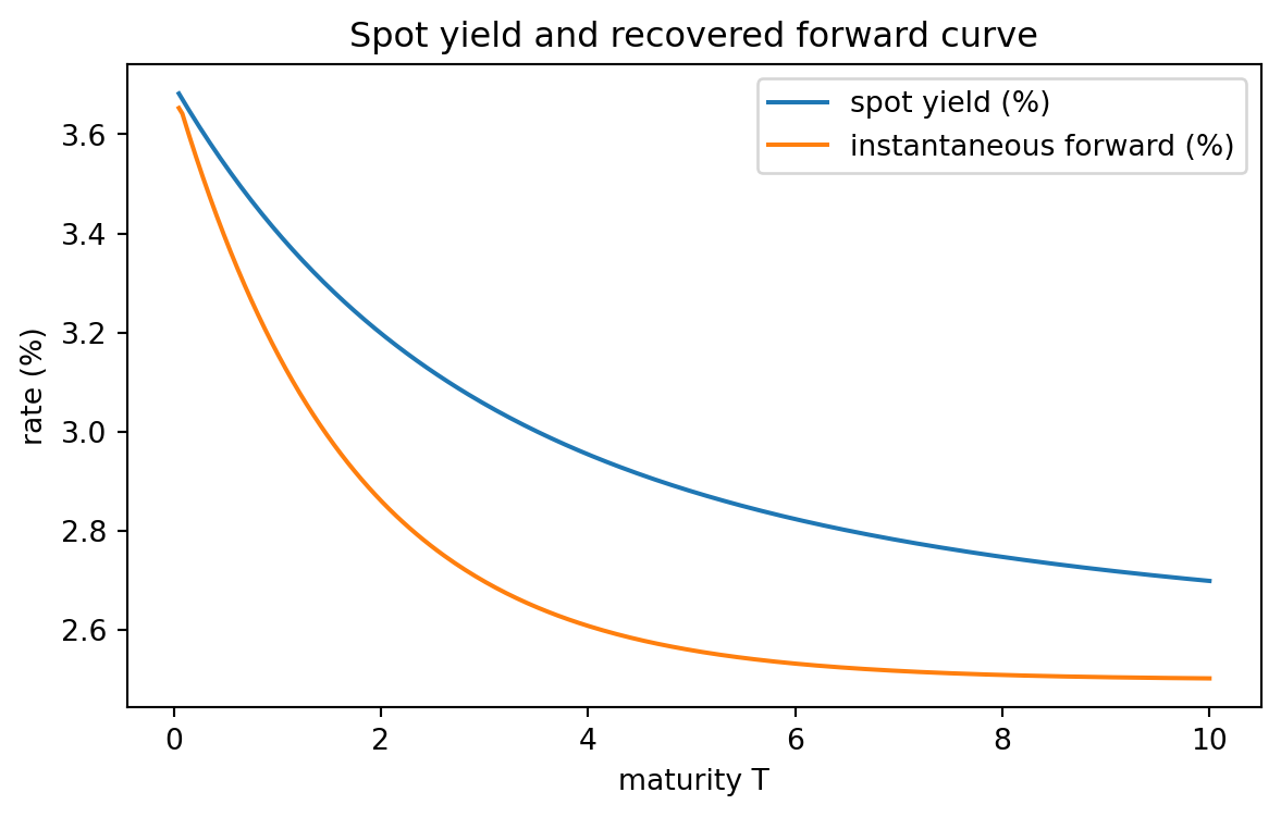
## 21.10 Python Example: Forward Rates from Bond Prices
The first computational task is to move between bond prices, spot rates, and forward rates.
```{python}
#| label: ch21-forward-from-discount
#| fig-cap: "Recovering forward rates from a smooth discount curve."
import numpy as np
import matplotlib.pyplot as plt

T = np.linspace(0.05, 10, 300)

# A synthetic continuously compounded spot curve.
y = 0.025 + 0.012 * (1 - np.exp(-0.6 * T)) / (0.6 * T)
P = np.exp(-y * T)

# The instantaneous forward rate is - d/dT log P(0,T).
logP = np.log(P)
f_numeric = -np.gradient(logP, T)

# Reconstruct discount factors from the numerical forward curve.
cum_int = np.zeros_like(T)
for i in range(1, len(T)):
    h = T[i] - T[i - 1]
    cum_int[i] = cum_int[i - 1] + 0.5 * h * (f_numeric[i] + f_numeric[i - 1])
P_reconstructed = np.exp(-cum_int)

plt.figure(figsize=(7, 4))
plt.plot(T, 100 * y, label="spot yield (%)")
plt.plot(T, 100 * f_numeric, label="instantaneous forward (%)")
plt.xlabel("maturity T")
plt.ylabel("rate (%)")
plt.title("Spot yield and recovered forward curve")
plt.legend()
plt.show()

print("Maximum discount reconstruction error:", np.max(np.abs(P - P_reconstructed)))
```
The reconstruction error is caused by numerical differentiation and integration. With a smoother grid, it becomes smaller.
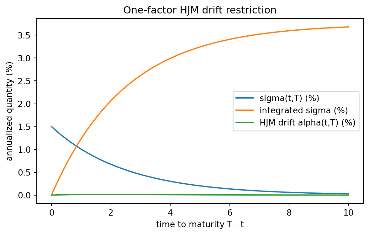
## 21.11 Python Example: HJM Drift from Volatility
The next example computes the one-factor HJM drift for an exponentially decaying volatility function.
```{python}
#| label: ch21-hjm-drift-python
#| fig-cap: "Volatility, integrated volatility, and HJM drift."
import numpy as np
import matplotlib.pyplot as plt

eta = 0.015
a = 0.40
tau = np.linspace(0, 10, 300)  # tau = T - t

sigma = eta * np.exp(-a * tau)
integrated_sigma = eta * (1 - np.exp(-a * tau)) / a
alpha = sigma * integrated_sigma

plt.figure(figsize=(7, 4))
plt.plot(tau, 100 * sigma, label="sigma(t,T) (%)")
plt.plot(tau, 100 * integrated_sigma, label="integrated sigma (%)")
plt.plot(tau, 100 * alpha, label="HJM drift alpha(t,T) (%)")
plt.xlabel("time to maturity T - t")
plt.ylabel("annualized quantity (%)")
plt.title("One-factor HJM drift restriction")
plt.legend()
plt.show()

print("maximum HJM drift:", alpha.max())
print("time to maturity at maximum drift:", tau[np.argmax(alpha)])
```
The drift is zero at $T=t$ because the integral from $t$ to $T$ has length zero. It also becomes small at very long maturities when the volatility decays quickly.
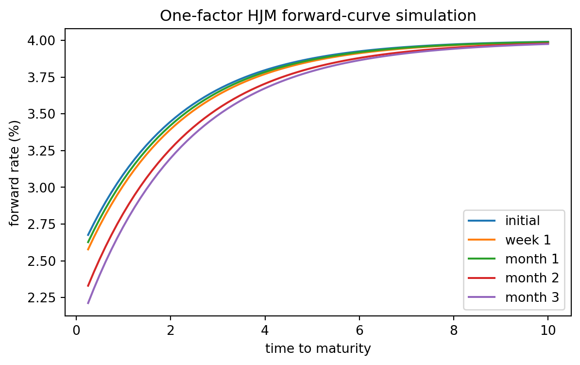
## 21.12 Python Example: Simulating a Discretized HJM Curve
To simulate an HJM model, we discretize the maturity axis. Let
$$
\tau_j=T_j-t,
\qquad j=0,1,\ldots,m.
$$
We simulate the forward curve under the risk-neutral measure by
$$
f_{n+1,j}
=
f_{n,j}+\alpha_j\Delta t+\sigma_j\Delta W_n.
$$
This simple discretization ignores the Musiela shift term, so it is best interpreted as a pedagogical fixed-maturity simulation over a short horizon. A production-quality term-structure simulation needs careful curve interpolation and aging.
```{python}
#| label: ch21-hjm-simulation
#| fig-cap: "Simulated HJM forward-rate curves under a one-factor volatility structure."
import numpy as np
import matplotlib.pyplot as plt

rng = np.random.default_rng(7243)

# Maturity grid measured from today.
tau = np.linspace(0.25, 10, 80)
dtau = tau[1] - tau[0]

# Initial forward curve.
f0 = 0.025 + 0.015 * (1 - np.exp(-0.5 * tau))

eta = 0.012
a = 0.35
sigma = eta * np.exp(-a * tau)

# Numerical integrated volatility int_0^tau sigma(u) du.
integrated_sigma = np.zeros_like(tau)
for j in range(1, len(tau)):
    integrated_sigma[j] = integrated_sigma[j - 1] + 0.5 * dtau * (sigma[j] + sigma[j - 1])
alpha = sigma * integrated_sigma

n_steps = 60
dt = 1 / 252
curves = [f0.copy()]
f = f0.copy()

for n in range(n_steps):
    dW = np.sqrt(dt) * rng.normal()
    f = f + alpha * dt + sigma * dW
    if n in [4, 19, 39, 59]:
        curves.append(f.copy())

plt.figure(figsize=(7, 4))
labels = ["initial", "week 1", "month 1", "month 2", "month 3"]
for curve, label in zip(curves, labels):
    plt.plot(tau, 100 * curve, label=label)
plt.xlabel("time to maturity")
plt.ylabel("forward rate (%)")
plt.title("One-factor HJM forward-curve simulation")
plt.legend()
plt.show()
```
Because the same Brownian shock affects all maturity points, the curve movements are highly correlated. Multi-factor HJM models are used when one wants level, slope, and curvature movements.
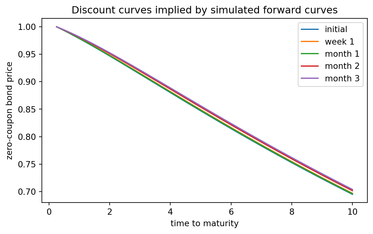
## 21.13 Python Example: Bond Prices from Simulated Forward Curves
Once the forward curve is known at time $t$, a zero-coupon bond price is computed by numerical integration:
$$
P(t,T)=\exp\left(-\int_t^T f(t,u)\,du\right).
$$
```{python}
#| label: ch21-bond-prices-from-forward-curves
#| fig-cap: "Discount curves generated from simulated forward curves."
import numpy as np
import matplotlib.pyplot as plt

# Reuse tau and curves from the previous example.

def discount_from_forward(tau_grid, forward_curve):
    integral = np.zeros_like(tau_grid)
    for j in range(1, len(tau_grid)):
        h = tau_grid[j] - tau_grid[j - 1]
        integral[j] = integral[j - 1] + 0.5 * h * (forward_curve[j] + forward_curve[j - 1])
    return np.exp(-integral)

plt.figure(figsize=(7, 4))
for curve, label in zip(curves, labels):
    P_curve = discount_from_forward(tau, curve)
    plt.plot(tau, P_curve, label=label)
plt.xlabel("time to maturity")
plt.ylabel("zero-coupon bond price")
plt.title("Discount curves implied by simulated forward curves")
plt.legend()
plt.show()
```
This example emphasizes the HJM workflow:
1. specify the initial forward curve;
2. specify forward-rate volatility;
3. compute no-arbitrage drift;
4. simulate the forward curve;
5. integrate the curve to price bonds.
## 21.14 Relation to Short-Rate Models
Every HJM model has a short rate
$$
r_t=f(t,t).
$$
But not every HJM model is conveniently represented by a finite-dimensional short-rate model.
A short-rate model is finite-dimensional when a small number of state variables are enough to describe the whole term structure. For example, affine short-rate models often produce bond prices of the form
$$
P(t,T)=A(t,T)e^{-B(t,T)r_t}.
$$
In a general HJM model, the future curve depends on the entire current curve, not just on a scalar short rate. This is why HJM is often described as an infinite-dimensional model.
::: {.remark}
## HJM contains short-rate models but is broader
Many classic interest-rate models can be embedded inside HJM by computing the forward-rate volatility they imply. The HJM framework is broader because it starts directly from forward-rate volatilities and enforces no-arbitrage at the curve level.
:::
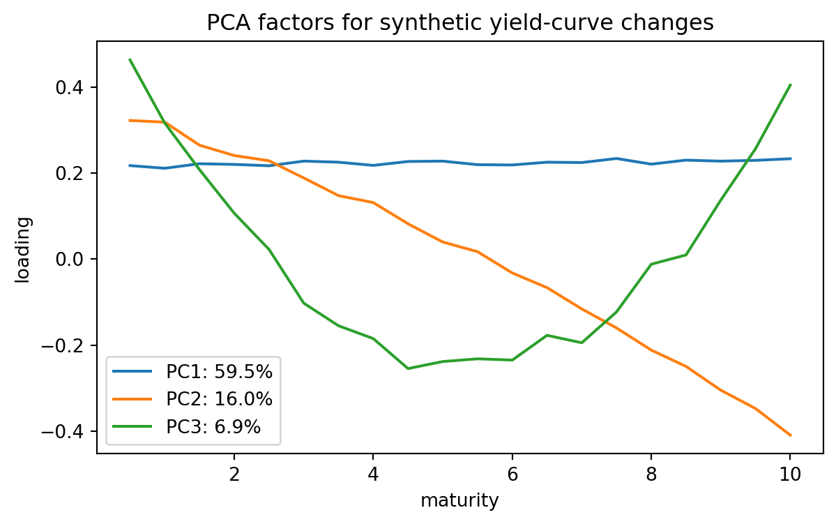
## 21.15 Calibration and Principal Components
In practice, yield-curve changes are often summarized by a small number of empirical factors:
- level changes;
- slope changes;
- curvature changes.
Principal component analysis is frequently used to estimate these dominant modes from historical yield changes. An HJM model can then use volatility functions that resemble these empirical factors.
```{python}
#| label: ch21-pca-yield-curve-changes
#| fig-cap: "Synthetic level, slope, and curvature factors recovered by PCA."
import numpy as np
import matplotlib.pyplot as plt

rng = np.random.default_rng(2026)

maturities = np.linspace(0.5, 10, 20)
n_days = 800

level = np.ones_like(maturities)
slope = maturities - maturities.mean()
slope = slope / np.linalg.norm(slope)
curvature = -(maturities - 5) ** 2
curvature = curvature - curvature.mean()
curvature = curvature / np.linalg.norm(curvature)
level = level / np.linalg.norm(level)

factors = np.vstack([level, slope, curvature])
vols = np.array([0.006, 0.003, 0.002])
Z = rng.normal(size=(n_days, 3)) * vols
noise = 0.0008 * rng.normal(size=(n_days, len(maturities)))
changes = Z @ factors + noise

# PCA by singular value decomposition.
X = changes - changes.mean(axis=0)
U, S, Vt = np.linalg.svd(X, full_matrices=False)
explained = S**2 / np.sum(S**2)

plt.figure(figsize=(7, 4))
for k in range(3):
    sign = 1 if Vt[k, 0] >= 0 else -1
    plt.plot(maturities, sign * Vt[k], label=f"PC{k+1}: {100*explained[k]:.1f}%")
plt.xlabel("maturity")
plt.ylabel("loading")
plt.title("PCA factors for synthetic yield-curve changes")
plt.legend()
plt.show()

print("Explained variance first three PCs:", explained[:3])
```
PCA is a statistical tool, not a no-arbitrage model by itself. HJM provides the no-arbitrage structure that can be combined with empirically estimated volatility factors.
## 21.16 Physical Measure versus Risk-Neutral Measure
As in equity models, there are two distinct modeling tasks.
Under the physical measure $\mathbb P$, we model historical curve evolution:
$$
df(t,T)=\alpha^{\mathbb P}(t,T)\,dt+
\sum_{k=1}^d \sigma_k(t,T)\,dW_t^{\mathbb P,k}.
$$
Under the risk-neutral measure $\mathbb Q$, we price bonds and derivatives:
$$
df(t,T)=\alpha^{\mathbb Q}(t,T)\,dt+
\sum_{k=1}^d \sigma_k(t,T)\,dW_t^{\mathbb Q,k}.
$$
The HJM drift restriction applies to $\alpha^{\mathbb Q}$. The physical drift $\alpha^{\mathbb P}$ is not determined by no-arbitrage alone.
The two measures are related by a market price of risk process. In a one-factor model, if
$$
dW_t^{\mathbb Q}=dW_t^{\mathbb P}+\lambda_t\,dt,
$$
then
$$
\alpha^{\mathbb P}(t,T)
=
\alpha^{\mathbb Q}(t,T)+\sigma(t,T)\lambda_t.
$$
This distinction is crucial:
- use $\mathbb P$ for forecasting and risk management;
- use $\mathbb Q$ for arbitrage-free pricing.
## 21.17 HJM Pricing of Interest-Rate Derivatives
An interest-rate derivative payoff may depend on future bond prices, future rates, or averages of rates. HJM gives a complete model for the future evolution of the curve, so one can price such derivatives by risk-neutral expectation:
$$
V_t
=
\mathbb E^{\mathbb Q}\left[
\exp\left(-\int_t^T r_s\,ds\right)X
\middle|\mathcal F_t
\right],
$$
where $X$ is the payoff at time $T$.
Examples include:
- bond options;
- caps and floors;
- swaptions;
- callable bonds;
- mortgage-backed securities.
Many of these products require numerical methods because the payoff depends on several points of the future yield curve.
## 21.18 Common Mistakes
::: {.warning}
## Common mistakes in HJM modeling
1. **Wrong sign in the forward-rate definition.** The correct formula is
$$f(t,T)=-\partial_T\log P(t,T).$$
2. **Forgetting that $r_t=f(t,t)$.** The short rate is the shortest-maturity forward rate.
3. **Choosing drift and volatility independently under $\mathbb Q$.** In risk-neutral HJM, no-arbitrage determines the drift from volatility.
4. **Confusing $T$ and $T-t$.** Calendar maturity and time to maturity are different. The Musiela parametrization uses $x=T-t$.
5. **Using historical drift for pricing.** Historical drift belongs to $\mathbb P$; no-arbitrage pricing uses $\mathbb Q$.
6. **Ignoring curve interpolation.** In computation, bond prices require integrals over the curve, so interpolation choices matter.
:::
## 21.19 AI-Assisted Learning Components
::: {.ai-box}
## AI prompt: check the HJM drift derivation
Ask an AI tool:
> Starting from $P(t,T)=\exp(-\int_t^T f(t,u)du)$ and $df(t,T)=\alpha(t,T)dt+\sigma(t,T)dW_t$, derive the HJM drift restriction. Identify every sign convention and every use of Itô's formula.
Then verify that the final answer is
$$
\alpha(t,T)=\sigma(t,T)\int_t^T \sigma(t,u)du.
$$
If the AI gives the negative of this expression, locate the sign error.
:::
::: {.ai-box}
## AI prompt: audit a simulation
Give an AI tool your HJM simulation code and ask:
> Does this code simulate fixed calendar maturities or time-to-maturity coordinates? Does it include the Musiela shift term? Which parts are appropriate for a textbook demonstration, and which parts would need improvement for production pricing?
The goal is not to outsource judgment, but to force a careful distinction between a pedagogical simulation and a robust numerical implementation.
:::
::: {.ai-box}
## AI prompt: compare short-rate and HJM models
Ask:
> Explain the difference between a short-rate model and an HJM model for an MS statistics student. Include the state variable, the no-arbitrage condition, and the computational implications.
Then rewrite the answer using precise mathematical notation.
:::
## 21.20 Exercises
### Conceptual exercises
1. Explain why the forward-rate curve contains more information than a single short rate.
2. Define $P(t,T)$, $y(t,T)$, and $f(t,T)$, and explain how they are related.
3. Why is the HJM state variable infinite-dimensional?
4. Explain in words what the HJM drift restriction means.
5. Why does the HJM drift restriction apply under $\mathbb Q$ rather than under $\mathbb P$?
### Mathematical exercises
6. Suppose $f(0,T)=a+bT+cT^2$. Derive $P(0,T)$ and $y(0,T)$.
7. Starting from $f(t,T)=-\partial_T\log P(t,T)$, show that
$$P(t,T)=\exp(-\int_t^T f(t,u)du).$$
8. Derive the one-factor HJM drift restriction carefully using Itô's formula.
9. In a two-factor model, prove that
$$\alpha(t,T)=\sum_{k=1}^2 \sigma_k(t,T)\int_t^T\sigma_k(t,u)du.$$
10. For $\sigma(t,T)=\eta e^{-a(T-t)}$, compute the HJM drift.
11. For constant volatility $\sigma(t,T)=\sigma_0$, compute the HJM drift and explain why it grows with maturity.
12. Show that the short rate satisfies $r_t=f(t,t)$.
### Computational exercises
13. Write a Python function that takes a forward curve on a grid and returns zero-coupon bond prices.
14. Write a Python function that approximates forward rates from observed zero-coupon bond prices.
15. Simulate a one-factor HJM model with constant volatility and compare the resulting forward curves with exponentially decaying volatility.
16. Numerically verify the HJM drift restriction by comparing
$$\int_t^T\alpha(t,u)du$$
with
$$\frac12\left(\int_t^T\sigma(t,u)du\right)^2.$$
17. Generate synthetic yield-curve changes and use PCA to estimate level, slope, and curvature factors.
### AI-assisted exercises
18. Ask an AI tool to derive the HJM drift restriction. Identify whether it uses the same sign convention as this chapter.
19. Ask an AI tool to produce Python code for HJM simulation. Audit whether the code uses $\mathbb P$ or $\mathbb Q$ dynamics.
20. Ask an AI tool to explain the Musiela parametrization. Improve the explanation by adding the shift term explicitly.
## 21.21 Chapter Summary
The HJM framework models the entire forward-rate curve rather than a single short rate. The fundamental relation
$$
P(t,T)=\exp\left(-\int_t^T f(t,u)\,du\right)
$$
connects forward rates to zero-coupon bond prices.
Under the risk-neutral measure, zero-coupon bonds must earn the short rate after discounting. This martingale requirement forces the HJM drift restriction. In the one-factor case,
$$
\alpha(t,T)=\sigma(t,T)\int_t^T\sigma(t,u)\,du.
$$
In the multi-factor case,
$$
\alpha(t,T)=\sum_{k=1}^d \sigma_k(t,T)\int_t^T\sigma_k(t,u)\,du.
$$
Thus HJM is a clean mathematical expression of no-arbitrage: choose the forward-rate volatility, and the risk-neutral drift is determined. This makes the framework a natural bridge between stochastic calculus, fixed-income pricing, functional data analysis, and modern computational finance.