---
title: "Chapter 25. Jump Models"
---
::: {.chapter-objectives}
## Learning Goals
By the end of this chapter, students should be able to:
- explain why continuous-path diffusion models miss sudden price moves;
- define Poisson processes, compound Poisson processes, and compensated Poisson martingales;
- derive the basic mean, variance, and moment-generating formulas for compound Poisson jumps;
- write stock-price dynamics with proportional jumps using left limits $S_{t-}$;
- distinguish jump sizes in price space from jump sizes in log-price space;
- derive the risk-neutral drift adjustment in a jump-diffusion model;
- state and use the Merton jump-diffusion model;
- price European options by risk-neutral Monte Carlo simulation and by conditioning on jump counts;
- formulate the pricing partial integro-differential equation for a jump-diffusion model;
- explain why jump risk usually makes markets incomplete;
- use Python and AI tools to audit notation, simulation code, and model assumptions.
:::
::: {.hero-box}
Black--Scholes paths are continuous. Real asset prices sometimes move discontinuously: an earnings announcement, a credit event, a central-bank surprise, a geopolitical shock, or a sudden liquidity event can move prices by several percent in a short time.
Jump models add a second source of randomness to the diffusion model. The diffusion part models many small shocks; the jump part models rare but large shocks:
$$
\frac{dS_t}{S_{t-}}
=
\mu\,dt+\sigma\,dW_t+(J-1)\,dN_t.
$$
The mathematical challenge is that the path is no longer continuous. The financial challenge is that jumps cannot usually be hedged away by continuous trading in the stock and money-market account.
:::
## 25.1 Why Add Jumps?
The Black--Scholes model assumes
$$
dS_t=\mu S_t\,dt+\sigma S_t\,dW_t.
$$
The solution has continuous sample paths. Therefore, over very small intervals, large moves are extremely unlikely under the normal increment assumption. For many liquid assets, however, historical return data and option prices suggest features that a pure diffusion model has difficulty reproducing:
1. **sudden discontinuous-looking moves** after news events;
2. **heavy tails** in short-horizon returns;
3. **short-maturity implied-volatility smiles**;
4. **gap risk** that cannot be removed by continuous delta hedging.
A jump model separates two kinds of uncertainty:
- ordinary continuous noise, represented by Brownian motion;
- rare event risk, represented by a counting process.
This chapter studies the simplest and most important jump building block: the Poisson process.
## 25.2 Poisson Processes
A Poisson process counts random event arrivals. In finance, the event might be a market shock, default event, earnings surprise, or liquidity jump.
::: {.definition}
## Poisson process
A counting process $(N_t)_{t\ge 0}$ is a **Poisson process with intensity** $\lambda>0$ if:
1. $N_0=0$;
2. $N_t$ has independent increments;
3. $N_t-N_s$ depends only on $t-s$;
4. for $0\le s<t$,
$$
N_t-N_s\sim \operatorname{Poisson}(\lambda(t-s)).
$$
:::
Thus,
$$
\mathbb P(N_t=n)=e^{-\lambda t}\frac{(\lambda t)^n}{n!},
\qquad n=0,1,2,\ldots.
$$
The parameter $\lambda$ is the expected number of jumps per unit time:
$$
\mathbb E[N_t]=\lambda t,
\qquad
\operatorname{Var}(N_t)=\lambda t.
$$
A small-time approximation is especially useful:
$$
\mathbb P(N_{t+\Delta t}-N_t=1)=\lambda\Delta t+o(\Delta t),
$$
and
$$
\mathbb P(N_{t+\Delta t}-N_t\ge 2)=o(\Delta t).
$$
This says that, over a very short time interval, either no jump occurs or one jump occurs, with probability approximately proportional to the interval length.
### Waiting times
Let $T_1$ be the first jump time:
$$
T_1=\inf\{t\ge 0:N_t\ge 1\}.
$$
Then
$$
\mathbb P(T_1>t)=\mathbb P(N_t=0)=e^{-\lambda t}.
$$
Therefore $T_1$ has an exponential distribution with rate $\lambda$.
More generally, the interarrival times
$$
T_1,
\quad T_2-T_1,
\quad T_3-T_2,
\ldots
$$
are independent exponential random variables with rate $\lambda$.
## 25.3 Compensated Poisson Martingales
The Poisson process has deterministic mean $\lambda t$. Subtracting this mean gives a martingale.
::: {.theorem}
## Compensated Poisson martingale
If $(N_t)$ is a Poisson process with intensity $\lambda$, then
$$
M_t=N_t-\lambda t
$$
is a martingale with respect to the natural filtration generated by $N$.
:::
### Proof idea
For $s<t$,
$$
\mathbb E[M_t\mid \mathcal F_s]
=
\mathbb E[N_t-\lambda t\mid \mathcal F_s].
$$
Using independent increments,
$$
\mathbb E[N_t\mid\mathcal F_s]
=
N_s+\mathbb E[N_t-N_s]
=
N_s+\lambda(t-s).
$$
Thus,
$$
\mathbb E[M_t\mid\mathcal F_s]
=
N_s+\lambda(t-s)-\lambda t
=
N_s-\lambda s
=
M_s.
$$
The compensated process $dN_t-\lambda dt$ plays a role similar to $dW_t$: it is a zero-mean random shock under the current information.
## 25.4 Compound Poisson Processes
A Poisson process tells us **when** jumps occur. A compound Poisson process also tells us **how large** the jumps are.
::: {.definition}
## Compound Poisson process
Let $(N_t)$ be a Poisson process with intensity $\lambda$. Let $Y_1,Y_2,\ldots$ be independent and identically distributed jump sizes, independent of $N$. The process
$$
X_t=\sum_{i=1}^{N_t}Y_i
$$
is called a **compound Poisson process**.
:::
If $N_t=0$, the sum is interpreted as zero. The process $X_t$ is piecewise constant and jumps by amount $Y_i$ at the $i$th jump time.
### Mean and variance
Using conditioning on $N_t$,
$$
\mathbb E[X_t\mid N_t=n]=n\mathbb E[Y_1].
$$
Therefore,
$$
\mathbb E[X_t]
=\mathbb E[N_t]\mathbb E[Y_1]
=\lambda t\,\mathbb E[Y_1].
$$
The variance is
$$
\operatorname{Var}(X_t)
=
\lambda t\,\mathbb E[Y_1^2].
$$
Equivalently,
$$
\operatorname{Var}(X_t)
=
\lambda t\left(\operatorname{Var}(Y_1)+(\mathbb E[Y_1])^2\right).
$$
The second term appears because randomness in the number of jumps creates additional variability.
### Moment-generating function
If $M_Y(u)=\mathbb E[e^{uY_1}]$, then
$$
\mathbb E[e^{uX_t}]
=
\exp\left(\lambda t(M_Y(u)-1)\right).
$$
This identity is one of the most useful formulas in jump modeling. It says that the cumulant-generating function of a compound Poisson process is linear in time.
## 25.5 Price Jumps and Log Jumps
A proportional jump model should keep stock prices positive. For this reason, it is common to write jumps multiplicatively.
Suppose that at a jump time, the stock price changes from $S_{t-}$ to $S_t$ according to
$$
S_t=S_{t-}J,
$$
where $J>0$ is the jump multiplier. The relative jump is
$$
\frac{S_t-S_{t-}}{S_{t-}}=J-1.
$$
The notation $S_{t-}$ means the left limit immediately before the jump:
$$
S_{t-}=\lim_{s\uparrow t}S_s.
$$
If we define the log-jump size by
$$
Y=\log J,
$$
then
$$
J=e^Y,
\qquad
S_t=S_{t-}e^Y.
$$
This distinction is important. A normal model for $Y$ gives positive jump multipliers $J=e^Y$, while a normal model directly for $J-1$ could produce invalid values below $-1$.
## 25.6 Jump-Diffusion Dynamics
A basic jump-diffusion stock model is
$$
\frac{dS_t}{S_{t-}}
=
\mu\,dt+\sigma\,dW_t+(J-1)\,dN_t.
$$
Here:
| Symbol | Meaning |
|---|---|
| $\mu$ | continuous drift parameter |
| $\sigma$ | diffusion volatility |
| $W_t$ | Brownian motion |
| $N_t$ | Poisson process with intensity $\lambda$ |
| $J$ | positive jump multiplier |
| $S_{t-}$ | pre-jump stock price |
If $dN_t=0$, then the local dynamics are diffusion-like:
$$
\frac{dS_t}{S_{t-}}=\mu\,dt+\sigma\,dW_t.
$$
If $dN_t=1$, then the stock is multiplied by $J$ at that instant.
### Explicit log solution
Assume that the jump multipliers are $J_i=e^{Y_i}$, where the $Y_i$ are independent and identically distributed. Then a solution has the form
$$
S_t
=
S_0
\exp\left(\left(\mu-\frac12\sigma^2\right)t+\sigma W_t+\sum_{i=1}^{N_t}Y_i\right).
$$
This formula makes the structure transparent:
- the Brownian part contributes a normal log-return;
- the jump part contributes a random sum of log-jump sizes.
## 25.7 Risk-Neutral Drift Adjustment
For pricing, we work under a risk-neutral measure $\mathbb Q$. Suppose the stock pays continuous dividend yield $q$. Under $\mathbb Q$, the discounted ex-dividend gain process should be a martingale.
Let
$$
\kappa=\mathbb E^{\mathbb Q}[J-1].
$$
The jump contribution has expected relative rate $\lambda\kappa$. Therefore, the risk-neutral jump-diffusion is usually written as
$$
\frac{dS_t}{S_{t-}}
=
(r-q-\lambda\kappa)\,dt+
\sigma\,dW_t^{\mathbb Q}+(J-1)\,dN_t^{\mathbb Q}.
$$
Taking conditional expectation over a small time interval gives
$$
\mathbb E^{\mathbb Q}\left[\frac{dS_t}{S_{t-}}\mid\mathcal F_t\right]
=
(r-q-\lambda\kappa)dt+
\lambda\kappa dt
=
(r-q)dt.
$$
Thus the expected total return rate under $\mathbb Q$ is $r-q$, as required by no-arbitrage pricing.
Equivalently, using the compensated Poisson martingale
$$
d\widetilde N_t=dN_t-\lambda dt,
$$
we can write
$$
\frac{dS_t}{S_{t-}}
=(r-q)\,dt+\sigma\,dW_t^{\mathbb Q}+(J-1)\,d\widetilde N_t^{\mathbb Q}.
$$
These two forms are mathematically equivalent, but the first form often makes simulation easier.
::: {.remark}
## Physical and risk-neutral jump parameters
The physical intensity and jump-size distribution need not equal their risk-neutral counterparts. Option prices contain information about market compensation for jump risk. Therefore, estimating jumps from historical returns and calibrating jumps from option prices are different problems.
:::
## 25.8 The Merton Jump-Diffusion Model
The Merton jump-diffusion model assumes that log-jump sizes are normally distributed:
$$
Y_i\sim N(m,\delta^2),
\qquad
J_i=e^{Y_i}.
$$
Then
$$
\kappa
=
\mathbb E[e^{Y_i}-1]
=
\exp\left(m+\frac12\delta^2\right)-1.
$$
Under $\mathbb Q$,
$$
S_T
=
S_0
\exp\left(
(r-q-\lambda\kappa-\frac12\sigma^2)T
+
\sigma W_T^{\mathbb Q}
+
\sum_{i=1}^{N_T}Y_i
\right).
$$
Conditional on $N_T=n$,
$$
\sum_{i=1}^{N_T}Y_i
\sim N(nm,n\delta^2).
$$
Therefore,
$$
\log S_T\mid (N_T=n)
\sim
N\left(
\log S_0+(r-q-\lambda\kappa-\frac12\sigma^2)T+nm,
\sigma^2T+n\delta^2
\right).
$$
This conditional normality is the key to efficient European option pricing in Merton's model.
## 25.9 Interactive Example: Poisson Arrivals and Compound Jumps
The following interactive demo shows a Poisson counting process and a compound Poisson jump process. The same jump times drive both plots; the lower plot also includes random jump sizes.
::: {.interactive-card}
### Poisson jumps and compound jump size
<div class="mf-control-row">
<label for="ch25-lambda">Jump intensity $\lambda$</label>
<input id="ch25-lambda" type="range" min="0.2" max="8.0" step="0.2" value="2.0">
<span id="ch25-lambda-val" class="mf-badge">2.0</span>
</div>
<div class="mf-control-row">
<label for="ch25-jumpscale">Jump-size scale</label>
<input id="ch25-jumpscale" type="range" min="0.02" max="0.30" step="0.01" value="0.10">
<span id="ch25-jumpscale-val" class="mf-badge">0.10</span>
</div>
<div id="ch25-poisson-demo" class="plotly-demo"></div>
<div id="ch25-poisson-output" class="mf-output"></div>
:::
<script>
mfPlotlyReady(function() {
var lambdaSlider = document.getElementById("ch25-lambda");
var scaleSlider = document.getElementById("ch25-jumpscale");
var lambdaVal = document.getElementById("ch25-lambda-val");
var scaleVal = document.getElementById("ch25-jumpscale-val");
var out = document.getElementById("ch25-poisson-output");
var plotId = "ch25-poisson-demo";
function lcg(seed) {
var m = 2147483647, a = 48271, state = seed % m;
return function() {
state = (a * state) % m;
return state / m;
};
}
function normalPair(u1, u2) {
var r = Math.sqrt(-2 * Math.log(Math.max(u1, 1e-12)));
var theta = 2 * Math.PI * u2;
return [r * Math.cos(theta), r * Math.sin(theta)];
}
function draw() {
var lambda = parseFloat(lambdaSlider.value);
var scale = parseFloat(scaleSlider.value);
lambdaVal.textContent = lambda.toFixed(1);
scaleVal.textContent = scale.toFixed(2);
var rand = lcg(25025);
var T = 1.0;
var t = [0.0];
var counts = [0];
var comp = [0.0];
var currentTime = 0.0;
var currentCount = 0;
var currentSum = 0.0;
while (currentTime < T) {
var u = Math.max(rand(), 1e-12);
var wait = -Math.log(u) / lambda;
currentTime += wait;
if (currentTime > T) break;
var z = normalPair(rand(), rand())[0];
var y = -0.03 + scale * z;
t.push(currentTime);
counts.push(currentCount);
comp.push(currentSum);
currentCount += 1;
currentSum += y;
t.push(currentTime);
counts.push(currentCount);
comp.push(currentSum);
}
t.push(T);
counts.push(currentCount);
comp.push(currentSum);
var traces = [
{x: t, y: counts, mode: "lines", line: {shape: "hv"}, name: "N_t", yaxis: "y"},
{x: t, y: comp, mode: "lines", line: {shape: "hv"}, name: "compound sum", yaxis: "y2"}
];
var layout = {
title: "Poisson counting process and compound Poisson process",
xaxis: {title: "time"},
yaxis: {title: "jump count"},
yaxis2: {title: "sum of log jumps", overlaying: "y", side: "right"},
margin: {l: 60, r: 65, t: 55, b: 50},
legend: {orientation: "h"}
};
Plotly.newPlot(plotId, traces, layout, {responsive: true});
out.innerHTML = "For this simulated path, $N_T = " + currentCount + "$. The theoretical mean is $\\lambda T = " + lambda.toFixed(1) + "$.";
}
lambdaSlider.addEventListener("input", draw);
scaleSlider.addEventListener("input", draw);
draw();
});
</script>
## 25.10 Python Example: Simulating a Poisson Process
```{python}
#| label: ch25-poisson-simulation
#| echo: true
#| warning: false
#| message: false
import math
import numpy as np
import matplotlib.pyplot as plt

rng = np.random.default_rng(25025)

lam = 3.0
T = 1.0
n_paths = 20_000

N_T = rng.poisson(lam * T, size=n_paths)

print("Sample mean:", N_T.mean())
print("Theoretical mean:", lam * T)
print("Sample variance:", N_T.var(ddof=1))
print("Theoretical variance:", lam * T)

plt.figure(figsize=(7, 4))
values = np.arange(0, N_T.max() + 1)
counts = np.bincount(N_T, minlength=len(values)) / n_paths
plt.bar(values, counts, alpha=0.75, label="simulation")
pmf = np.exp(-lam*T) * np.array([(lam*T)**k / math.factorial(int(k)) for k in values])
plt.plot(values, pmf, marker="o", label="Poisson pmf")
plt.xlabel("number of jumps by T")
plt.ylabel("probability")
plt.title("Poisson distribution of jump counts")
plt.legend()
plt.show()
```
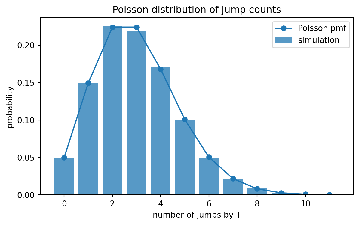
The mean and variance are both close to $\lambda T$. This equality is a useful diagnostic when checking Poisson simulation code.
## 25.11 Python Example: Compound Poisson Mean and Variance
```{python}
#| label: ch25-compound-poisson
#| echo: true
#| warning: false
#| message: false
import numpy as np

rng = np.random.default_rng(25026)

lam = 4.0
T = 1.0
m = -0.02
delta = 0.10
n_paths = 100_000

N = rng.poisson(lam * T, size=n_paths)
X = np.zeros(n_paths)

for i, n in enumerate(N):
    if n > 0:
        X[i] = rng.normal(m, delta, size=n).sum()

EY = m
EY2 = delta**2 + m**2

print("Simulated E[X_T]:", X.mean())
print("Theory E[X_T]:", lam * T * EY)
print("Simulated Var[X_T]:", X.var(ddof=1))
print("Theory Var[X_T]:", lam * T * EY2)
```
The variance formula uses $\mathbb E[Y^2]$, not merely $\operatorname{Var}(Y)$.
## 25.12 Risk-Neutral Pricing of a European Claim
Let $H=h(S_T)$ be a European payoff. Under a risk-neutral measure $\mathbb Q$,
$$
V_0=e^{-rT}\mathbb E^{\mathbb Q}[h(S_T)].
$$
For a European call,
$$
h(S_T)=(S_T-K)^+.
$$
In the Merton jump-diffusion model,
$$
C_0=e^{-rT}\mathbb E^{\mathbb Q}[(S_T-K)^+].
$$
The expectation may be computed by Monte Carlo or by conditioning on the number of jumps $N_T$.
### Conditional lognormal pricing
Conditional on $N_T=n$, write
$$
\log S_T\mid N_T=n\sim N(a_n,b_n^2),
$$
where
$$
a_n=\log S_0+(r-q-\lambda\kappa-\frac12\sigma^2)T+nm,
$$
and
$$
b_n^2=\sigma^2T+n\delta^2.
$$
If $X\sim N(a,b^2)$, then
$$
\mathbb E[(e^X-K)^+]
=
\exp(a+\frac12b^2)\Phi\left(\frac{a+b^2-\log K}{b}\right)
-
K\Phi\left(\frac{a-\log K}{b}\right).
$$
Therefore,
$$
C_0
=
e^{-rT}\sum_{n=0}^{\infty}
\mathbb P(N_T=n)
\left[
\exp(a_n+\frac12b_n^2)\Phi(d_{1,n})
-
K\Phi(d_{2,n})
\right],
$$
where
$$
d_{1,n}=\frac{a_n+b_n^2-\log K}{b_n},
\qquad
d_{2,n}=\frac{a_n-\log K}{b_n}.
$$
This formula is often easier to explain to students than quoting a closed-form series directly: first condition on the jump count, then apply a lognormal payoff identity.
## 25.13 Python Example: Merton Jump-Diffusion Paths
```{python}
#| label: ch25-merton-paths
#| echo: true
#| warning: false
#| message: false
import numpy as np
import matplotlib.pyplot as plt

rng = np.random.default_rng(25027)

S0 = 100.0
r = 0.03
q = 0.00
sigma = 0.18
lam = 1.2
m = -0.08
delta = 0.18
T = 1.0
steps = 252
n_paths = 8

dt = T / steps
kappa = np.exp(m + 0.5 * delta**2) - 1.0

S = np.full((n_paths, steps + 1), S0)
for t in range(1, steps + 1):
    Z = rng.normal(size=n_paths)
    dN = rng.poisson(lam * dt, size=n_paths)
    jump_sum = np.zeros(n_paths)
    for i, n in enumerate(dN):
        if n > 0:
            jump_sum[i] = rng.normal(m, delta, size=n).sum()
    log_increment = (r - q - lam*kappa - 0.5*sigma**2)*dt + sigma*np.sqrt(dt)*Z + jump_sum
    S[:, t] = S[:, t-1] * np.exp(log_increment)

time = np.linspace(0, T, steps + 1)

plt.figure(figsize=(8, 4))
for i in range(n_paths):
    plt.plot(time, S[i])
plt.xlabel("time")
plt.ylabel("stock price")
plt.title("Merton jump-diffusion sample paths")
plt.show()
```
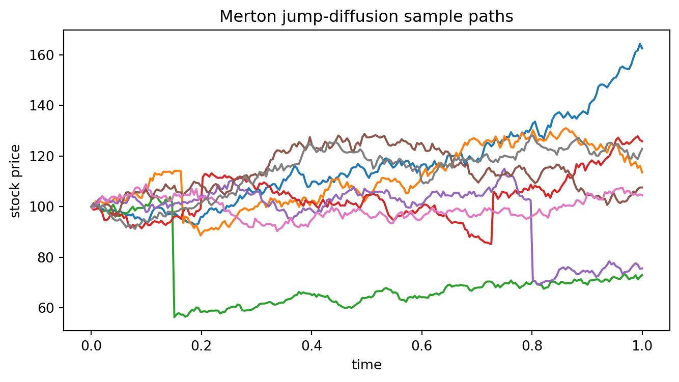
The paths combine continuous Brownian movement with occasional discontinuous jumps.
## 25.14 Python Example: Monte Carlo Option Pricing
```{python}
#| label: ch25-merton-monte-carlo
#| echo: true
#| warning: false
#| message: false
import numpy as np

rng = np.random.default_rng(25028)

S0 = 100.0
K = 100.0
r = 0.03
q = 0.00
sigma = 0.18
lam = 1.2
m = -0.08
delta = 0.18
T = 1.0
n_paths = 250_000

kappa = np.exp(m + 0.5 * delta**2) - 1.0
N = rng.poisson(lam * T, size=n_paths)
Z = rng.normal(size=n_paths)

jump_sum = np.zeros(n_paths)
for i, n in enumerate(N):
    if n > 0:
        jump_sum[i] = rng.normal(m, delta, size=n).sum()

log_ST = (
    np.log(S0)
    + (r - q - lam*kappa - 0.5*sigma**2)*T
    + sigma*np.sqrt(T)*Z
    + jump_sum
)
ST = np.exp(log_ST)
payoff = np.maximum(ST - K, 0.0)
price = np.exp(-r*T) * payoff.mean()
standard_error = np.exp(-r*T) * payoff.std(ddof=1) / np.sqrt(n_paths)

print("Monte Carlo price:", price)
print("Monte Carlo standard error:", standard_error)
print("Average discounted stock:", np.exp(-r*T) * ST.mean())
print("Theoretical forward-consistency target:", S0 * np.exp(-q*T))
```
The discounted expected stock price should be close to $S_0e^{-qT}$. This is a simple no-arbitrage diagnostic for the drift adjustment.
## 25.15 Python Example: Conditional Series Price
```{python}
#| label: ch25-merton-series
#| echo: true
#| warning: false
#| message: false
import math
import numpy as np

def Phi(x):
    return 0.5 * (1.0 + math.erf(x / math.sqrt(2.0)))

def lognormal_call_from_normal(a, b2, K):
    b = math.sqrt(max(b2, 1e-16))
    d1 = (a + b2 - math.log(K)) / b
    d2 = (a - math.log(K)) / b
    return math.exp(a + 0.5*b2) * Phi(d1) - K * Phi(d2)

def merton_call_series(S0, K, r, q, sigma, lam, m, delta, T, n_max=60):
    kappa = math.exp(m + 0.5*delta**2) - 1.0
    total = 0.0
    meanN = lam * T
    for n in range(n_max + 1):
        prob = math.exp(-meanN) * meanN**n / math.factorial(n)
        a = math.log(S0) + (r - q - lam*kappa - 0.5*sigma**2)*T + n*m
        b2 = sigma**2*T + n*delta**2
        total += prob * lognormal_call_from_normal(a, b2, K)
    return math.exp(-r*T) * total

price_series = merton_call_series(
    S0=100.0,
    K=100.0,
    r=0.03,
    q=0.00,
    sigma=0.18,
    lam=1.2,
    m=-0.08,
    delta=0.18,
    T=1.0,
    n_max=60
)

print("Merton conditional-series price:", price_series)
```
The conditional-series method removes much of the Monte Carlo noise by analytically integrating over the Brownian and jump-size randomness conditional on the jump count.
## 25.16 Interactive Example: Jump Intensity and Option Prices
The next demo prices a European call by the conditional-series formula. It shows how jump intensity and average jump size change option value and the distribution of terminal prices.
::: {.interactive-card}
### Merton jump-diffusion call price
<div class="mf-control-row">
<label for="ch25-price-lambda">Jump intensity $\lambda$</label>
<input id="ch25-price-lambda" type="range" min="0.0" max="4.0" step="0.1" value="1.0">
<span id="ch25-price-lambda-val" class="mf-badge">1.0</span>
</div>
<div class="mf-control-row">
<label for="ch25-price-m">Mean log jump $m$</label>
<input id="ch25-price-m" type="range" min="-0.30" max="0.10" step="0.01" value="-0.08">
<span id="ch25-price-m-val" class="mf-badge">-0.08</span>
</div>
<div class="mf-control-row">
<label for="ch25-price-delta">Jump volatility $\delta$</label>
<input id="ch25-price-delta" type="range" min="0.01" max="0.45" step="0.01" value="0.18">
<span id="ch25-price-delta-val" class="mf-badge">0.18</span>
</div>
<div id="ch25-merton-price-demo" class="plotly-demo"></div>
<div id="ch25-merton-price-output" class="mf-output"></div>
:::
<script>
mfPlotlyReady(function() {
var lambdaSlider = document.getElementById("ch25-price-lambda");
var mSlider = document.getElementById("ch25-price-m");
var deltaSlider = document.getElementById("ch25-price-delta");
var lambdaVal = document.getElementById("ch25-price-lambda-val");
var mVal = document.getElementById("ch25-price-m-val");
var deltaVal = document.getElementById("ch25-price-delta-val");
var out = document.getElementById("ch25-merton-price-output");
var plotId = "ch25-merton-price-demo";
function erf(x) {
var sign = x >= 0 ? 1 : -1;
x = Math.abs(x);
var a1 = 0.254829592, a2 = -0.284496736, a3 = 1.421413741;
var a4 = -1.453152027, a5 = 1.061405429, p = 0.3275911;
var t = 1.0 / (1.0 + p * x);
var y = 1.0 - (((((a5 * t + a4) * t) + a3) * t + a2) * t + a1) * t * Math.exp(-x * x);
return sign * y;
}
function Phi(x) {
return 0.5 * (1.0 + erf(x / Math.sqrt(2.0)));
}
function factorial(n) {
var f = 1;
for (var i = 2; i <= n; i++) f *= i;
return f;
}
function lognormalCall(a, b2, K) {
var b = Math.sqrt(Math.max(b2, 1e-16));
var d1 = (a + b2 - Math.log(K)) / b;
var d2 = (a - Math.log(K)) / b;
return Math.exp(a + 0.5*b2) * Phi(d1) - K * Phi(d2);
}
function mertonCall(S0, K, r, q, sigma, lambda, m, delta, T) {
var kappa = Math.exp(m + 0.5*delta*delta) - 1.0;
var meanN = lambda * T;
var total = 0.0;
for (var n = 0; n <= 40; n++) {
var prob = Math.exp(-meanN) * Math.pow(meanN, n) / factorial(n);
var a = Math.log(S0) + (r - q - lambda*kappa - 0.5*sigma*sigma)*T + n*m;
var b2 = sigma*sigma*T + n*delta*delta;
total += prob * lognormalCall(a, b2, K);
}
return Math.exp(-r*T) * total;
}
function draw() {
var lambda = parseFloat(lambdaSlider.value);
var m = parseFloat(mSlider.value);
var delta = parseFloat(deltaSlider.value);
lambdaVal.textContent = lambda.toFixed(1);
mVal.textContent = m.toFixed(2);
deltaVal.textContent = delta.toFixed(2);
var S0 = 100.0, r = 0.03, q = 0.00, sigma = 0.18, T = 1.0;
var strikes = [];
var prices = [];
var bsPrices = [];
for (var K = 60; K <= 140; K += 2) {
strikes.push(K);
prices.push(mertonCall(S0, K, r, q, sigma, lambda, m, delta, T));
bsPrices.push(mertonCall(S0, K, r, q, sigma, 0.0, 0.0, 0.01, T));
}
var atm = mertonCall(S0, 100.0, r, q, sigma, lambda, m, delta, T);
var traces = [
{x: strikes, y: prices, mode: "lines", name: "jump-diffusion call"},
{x: strikes, y: bsPrices, mode: "lines", name: "no-jump benchmark", line: {dash: "dot"}}
];
var layout = {
title: "European call prices under a Merton jump-diffusion",
xaxis: {title: "strike K"},
yaxis: {title: "call price"},
margin: {l: 65, r: 20, t: 55, b: 50},
legend: {orientation: "h"}
};
Plotly.newPlot(plotId, traces, layout, {responsive: true});
var kappa = Math.exp(m + 0.5*delta*delta) - 1.0;
out.innerHTML = "ATM call price: <strong>" + atm.toFixed(4) + "</strong>. The jump compensator is $\\kappa = " + kappa.toFixed(4) + "$, so the drift adjustment is $-\\lambda\\kappa = " + (-lambda*kappa).toFixed(4) + "$.";
}
lambdaSlider.addEventListener("input", draw);
mSlider.addEventListener("input", draw);
deltaSlider.addEventListener("input", draw);
draw();
});
</script>
## 25.17 Pricing PIDE for Jump-Diffusions
Let $V(t,S)$ be the price of a European claim. Under the risk-neutral jump-diffusion
$$
\frac{dS_t}{S_{t-}}
=
(r-q-\lambda\kappa)\,dt+\sigma\,dW_t+(J-1)\,dN_t,
$$
the infinitesimal generator applied to a smooth test function $f$ is
$$
\mathcal A f(s)
=
(r-q-\lambda\kappa)s f_s(s)
+
\frac12\sigma^2s^2 f_{ss}(s)
+
\lambda\mathbb E[f(sJ)-f(s)].
$$
The pricing equation is therefore
$$
V_t+\mathcal A V-rV=0,
$$
or explicitly,
$$
V_t
+(r-q-\lambda\kappa)S V_S
+\frac12\sigma^2S^2V_{SS}
-rV
+\lambda\mathbb E[V(t,SJ)-V(t,S)]
=0.
$$
The terminal condition for a European call is
$$
V(T,S)=(S-K)^+.
$$
This equation is called a **partial integro-differential equation** because it contains both differential terms and an expectation over the jump-size distribution.
## 25.18 Incompleteness and Jump Risk
In Black--Scholes, one Brownian risk source is hedged by one risky asset plus the money-market account. In a jump-diffusion model, there are at least two sources of uncertainty:
1. Brownian diffusion risk;
2. jump arrival and jump-size risk.
A continuously rebalanced stock-and-bond strategy can hedge small Brownian movements locally, but it cannot generally hedge an unexpected jump of unknown size. This creates market incompleteness.
::: {.important}
## Why jumps usually break perfect replication
Delta hedging cancels the first-order continuous term $dW_t$. It does not cancel the discontinuous jump term
$$
V(t,S_{t-}J)-V(t,S_{t-})-\Delta S_{t-}(J-1).
$$
Unless the payoff is linear in $S$ or enough additional traded instruments are available, jump risk remains unhedged.
:::
Because of incompleteness, the risk-neutral measure may not be unique. Modelers often choose a risk-neutral jump intensity and jump-size distribution by calibration to liquid option prices.
## 25.19 Jump Risk and Delta Hedging Error
For a smooth option price $V(t,S)$, the continuous Black--Scholes delta is
$$
\Delta=V_S(t,S).
$$
If the stock jumps from $S$ to $SJ$, the option value jumps from $V(t,S)$ to $V(t,SJ)$. The stock hedge changes by approximately
$$
\Delta(SJ-S)=\Delta S(J-1).
$$
The jump hedging error is therefore
$$
\varepsilon_J
=
V(t,SJ)-V(t,S)-V_S(t,S)S(J-1).
$$
For nonlinear payoffs, this is usually not zero. This formula is one of the clearest mathematical explanations of gap risk.
## 25.20 Python Example: Jump Tails versus Diffusion Tails
```{python}
#| label: ch25-tail-comparison
#| echo: true
#| warning: false
#| message: false
import numpy as np
import matplotlib.pyplot as plt

rng = np.random.default_rng(25029)

S0 = 100.0
r = 0.03
sigma = 0.18
lam = 1.2
m = -0.08
delta = 0.18
T = 1.0
n = 200_000

# No-jump log returns
Z = rng.normal(size=n)
logret_diffusion = (r - 0.5*sigma**2)*T + sigma*np.sqrt(T)*Z

# Jump-diffusion log returns under risk-neutral drift adjustment
kappa = np.exp(m + 0.5*delta**2) - 1.0
N = rng.poisson(lam*T, size=n)
jump_sum = np.zeros(n)
for i, count in enumerate(N):
    if count > 0:
        jump_sum[i] = rng.normal(m, delta, size=count).sum()
logret_jump = (r - lam*kappa - 0.5*sigma**2)*T + sigma*np.sqrt(T)*rng.normal(size=n) + jump_sum

for name, x in [("diffusion", logret_diffusion), ("jump diffusion", logret_jump)]:
    qs = np.quantile(x, [0.01, 0.05, 0.50, 0.95, 0.99])
    print(name, qs)

plt.figure(figsize=(8, 4))
plt.hist(logret_diffusion, bins=120, density=True, alpha=0.45, label="diffusion")
plt.hist(logret_jump, bins=120, density=True, alpha=0.45, label="jump diffusion")
plt.xlabel("log return")
plt.ylabel("density")
plt.title("Jump diffusion can generate heavier tails")
plt.legend()
plt.show()
```
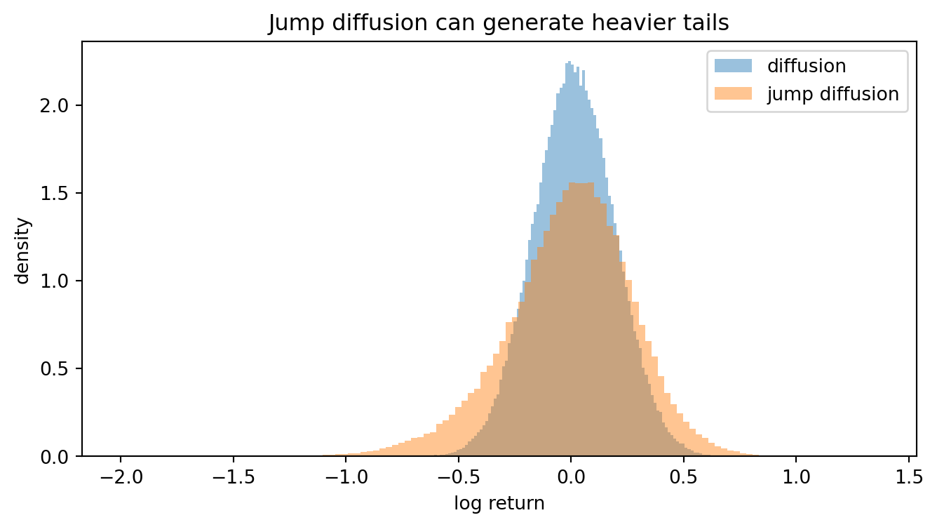
The jump model can assign more probability to large negative and positive outcomes, depending on jump parameters.
## 25.21 Model Calibration and Interpretation
A Merton jump-diffusion has several parameters:
$$
(r,q,\sigma,\lambda,m,\delta).
$$
The parameters $(\lambda,m,\delta)$ control jump behavior:
- $\lambda$ controls how often jumps occur;
- $m$ controls the average log-jump direction;
- $\delta$ controls dispersion in jump size.
In practice, historical data may have too few observed jumps to estimate these parameters precisely. Option prices, especially short-maturity out-of-the-money options, can contain additional information about market-implied jump risk.
This creates a statistical issue: many parameter combinations can produce similar option prices. Calibration is therefore an inverse problem and should be regularized, constrained, and checked for stability.
## 25.22 AI-Assisted Learning Components
### AI prompt: distinguish jump-size conventions
Ask an AI tool:
> In a Merton jump-diffusion model, explain the difference between modeling the jump multiplier $J$, the relative jump $J-1$, and the log-jump $Y=\log J$. Give one reason why modeling $Y$ as normal is mathematically convenient.
Then check that the answer clearly states that $J=e^Y>0$.
### AI prompt: audit a risk-neutral drift
Give an AI tool the formula
$$
\frac{dS_t}{S_{t-}}=r\,dt+\sigma\,dW_t+(J-1)dN_t
$$
and ask:
> Is this risk-neutral stock model correctly compensated? If not, what drift adjustment is missing?
A correct response should identify the missing $-\lambda\kappa$ adjustment, where $\kappa=\mathbb E^{\mathbb Q}[J-1]$.
### AI prompt: code review for simulations
Ask an AI tool to review Merton simulation code and check whether:
1. the Poisson jump count uses mean $\lambda\Delta t$ per step;
2. multiple jumps per time step are handled or intentionally approximated;
3. the log-jump sum is added to the log return;
4. the drift includes $-\lambda\kappa$ under the risk-neutral measure;
5. the discounted expected stock price is close to $S_0e^{-qT}$.
## 25.23 Common Mistakes
1. **Forgetting $S_{t-}$.** Jump equations use the pre-jump price because the jump size multiplies the price just before the jump.
2. **Confusing $J$ and $Y$.** If $Y$ is a log jump, then the multiplier is $J=e^Y$.
3. **Omitting the compensator.** Under $\mathbb Q$, the drift must account for expected jump returns.
4. **Treating delta hedging as exact.** Delta hedging does not eliminate jump-size risk.
5. **Estimating and calibrating as if they were the same.** Historical jump parameters and risk-neutral jump parameters need not agree.
6. **Allowing impossible price jumps.** A model for relative jumps must avoid values below $-1$.
## 25.24 Exercises
### Conceptual exercises
1. Explain why Brownian diffusion models have continuous paths and why this can be unrealistic at short horizons.
2. Give two financial examples of events that might be modeled as jumps.
3. Explain the difference between a Poisson process and a compound Poisson process.
4. Why is $N_t-\lambda t$ a martingale but $N_t$ is not?
5. What is the financial meaning of the jump compensator $\lambda\kappa$?
### Mathematical exercises
6. Prove that $\mathbb E[N_t]=\lambda t$ and $\operatorname{Var}(N_t)=\lambda t$.
7. Let $X_t=\sum_{i=1}^{N_t}Y_i$. Derive $\mathbb E[X_t]$ by conditioning on $N_t$.
8. Derive $\operatorname{Var}(X_t)=\lambda t\mathbb E[Y^2]$ using the law of total variance.
9. If $Y\sim N(m,\delta^2)$, show that $\mathbb E[e^Y-1]=e^{m+\delta^2/2}-1$.
10. Starting from the risk-neutral jump-diffusion, verify that $\mathbb E^{\mathbb Q}[dS_t/S_{t-}\mid\mathcal F_t]=(r-q)dt$.
### Pricing exercises
11. Derive the conditional distribution of $\log S_T$ given $N_T=n$ in the Merton model.
12. Prove the lognormal call identity used in the conditional-series pricing formula.
13. Write the PIDE for a European put option under the Merton jump-diffusion model.
14. Explain why a jump-diffusion market with only stock and bond is usually incomplete.
15. Compute the jump hedging error for a European call if the stock jumps from $S$ to $SJ$.
### Python exercises
16. Simulate a Poisson process by exponential waiting times and compare it with direct Poisson sampling of $N_T$.
17. Simulate a compound Poisson process with normal jump sizes and verify its mean and variance.
18. Implement a Merton jump-diffusion simulator using daily time steps.
19. Compare Monte Carlo and conditional-series European call prices.
20. Study how the call price changes as $\lambda$, $m$, and $\delta$ vary.
### AI-assisted exercises
21. Ask an AI tool to explain the difference between physical and risk-neutral jump intensity. Critique whether it distinguishes estimation from calibration.
22. Ask an AI tool to derive the Merton risk-neutral drift adjustment. Check each expectation step.
23. Ask an AI tool to review your simulation code and identify whether it works in price space or log-price space.
24. Ask an AI tool to explain why jumps create incomplete markets. Require a mathematical explanation using hedging error.
## 25.25 Chapter Summary
Jump models extend diffusion models by adding rare discontinuous moves. The Poisson process models the number of jumps, while a compound Poisson process models both jump times and jump sizes. In proportional stock-price models, jumps are naturally represented by positive multipliers $J=e^Y$.
The key risk-neutral adjustment is
$$
\frac{dS_t}{S_{t-}}
=
(r-q-\lambda\kappa)dt+
\sigma dW_t^{\mathbb Q}+(J-1)dN_t^{\mathbb Q},
\qquad
\kappa=\mathbb E^{\mathbb Q}[J-1].
$$
This adjustment ensures that the expected total return under $\mathbb Q$ is $r-q$. The Merton jump-diffusion model assumes normally distributed log jumps and leads to a conditionally lognormal terminal stock price. European option prices can be computed by Monte Carlo simulation or by conditioning on the jump count.
Mathematically, jump models introduce partial integro-differential equations and market incompleteness. Financially, they explain gap risk, short-maturity smile behavior, and the limitations of continuous delta hedging.