---
title: "Chapter 15. Black--Scholes Model"
---
::: {.chapter-objectives}
## Learning Goals
By the end of this chapter, students should be able to:
- state the Black--Scholes market model with a stock, a money-market account, and Brownian information;
- distinguish the physical measure from the pricing measure;
- define self-financing trading strategies in continuous time;
- apply Itô's formula to a derivative price $V(t,S_t)$;
- derive the Black--Scholes partial differential equation by delta hedging;
- interpret each term in the Black--Scholes PDE mathematically and financially;
- connect replication, no-arbitrage, martingales, and PDE methods;
- understand terminal and boundary conditions for European claims;
- explain why the drift $\mu$ disappears from the pricing PDE;
- recognize the assumptions and limitations of the Black--Scholes model;
- use Python and AI tools to check formulas, simulate hedging, and audit model assumptions.
:::
::: {.hero-box}
The Black--Scholes model is the first continuous-time model in which option prices can be derived from **replication** rather than from subjective beliefs about expected returns.
The market consists of a money-market account
$$
dB_t=rB_t\,dt,
$$
and a stock price
$$
dS_t=\mu S_t\,dt+\sigma S_t\,dW_t.
$$
If a European derivative has price $V(t,S)$, then no-arbitrage and continuous rebalancing lead to the Black--Scholes PDE
$$
V_t+\frac12\sigma^2S^2V_{SS}+rSV_S-rV=0.
$$
The striking point is that the physical drift $\mu$ does not appear in the PDE. Pricing depends on what can be replicated, not on what investors believe the stock will earn on average.
:::
## 15.1 Why This Model Matters
In the binomial model, we priced a derivative by dynamically choosing a number of shares and a bond position so that the final payoff was replicated in every state. The Black--Scholes model is the continuous-time limit of that idea.
The central question is:
> Can we construct a continuously rebalanced portfolio of stock and cash that has exactly the same payoff as a derivative?
If the answer is yes, then the derivative price must equal the cost of the replicating strategy. Otherwise, one could buy the cheaper object, sell the more expensive object, and lock in an arbitrage.
The key mathematical mechanism is Itô's formula. If the derivative value is
$$
V_t^{\text{derivative}}=V(t,S_t),
$$
then the stochastic differential of $V(t,S_t)$ contains a $dW_t$ term. By holding the correct number of stock shares, that random term can be canceled. This cancellation is called **delta hedging**.
::: {.callout-note}
## Main idea
The Black--Scholes PDE is not first a formula for a call option. It is first a **no-arbitrage condition** for every sufficiently smooth derivative price function in a complete continuous-time market.
:::
## 15.2 The Black--Scholes Market
We work on a filtered probability space
$$
(\Omega,F,(F_t)_{0\le t\le T},\mathbb P),
$$
where $W_t$ is a Brownian motion adapted to the filtration $(F_t)$. The filtration represents the market information observed through time.
The market contains two traded assets.
First, the money-market account satisfies
$$
dB_t=rB_t\,dt, \qquad B_0=1,
$$
where $r$ is a constant continuously compounded risk-free rate. Therefore
$$
B_t=e^{rt}.
$$
Second, the stock price follows geometric Brownian motion under the physical measure $\mathbb P$:
$$
dS_t=\mu S_t\,dt+\sigma S_t\,dW_t, \qquad S_0>0,
$$
where $\mu\in\mathbb R$ and $\sigma>0$ are constants.
The explicit solution is
$$
S_t=S_0\exp\left[\left(\mu-\frac12\sigma^2\right)t+\sigma W_t\right].
$$
::: {.definition}
### Definition 15.1: Black--Scholes market model
The Black--Scholes market model consists of a money-market account $B_t$ and a stock price $S_t$ satisfying
$$
dB_t=rB_t\,dt,
$$
and
$$
dS_t=\mu S_t\,dt+\sigma S_t\,dW_t,
$$
with constant $r$, $\mu$, and $\sigma>0$.
:::
The constants have different roles:
- $r$ is the return of the riskless asset;
- $\mu$ is the physical expected return of the stock;
- $\sigma$ is the stock volatility;
- $W_t$ is the Brownian source of uncertainty;
- $F_t$ is the information available to traders at time $t$.
## 15.3 Claims and Price Functions
A European derivative with maturity $T$ has a payoff
$$
H=h(S_T),
$$
where $h$ is a payoff function. For example, a European call option has
$$
h(S_T)=(S_T-K)^+,
$$
and a European put option has
$$
h(S_T)=(K-S_T)^+.
$$
In the Markovian Black--Scholes model, the derivative price at time $t$ is assumed to be a deterministic function of time and the current stock price:
$$
\text{price at time }t=V(t,S_t).
$$
The terminal condition is
$$
V(T,S)=h(S).
$$
The mathematical problem is therefore to determine a function
$$
V:[0,T]\times(0,\infty)\to\mathbb R
$$
such that $V(T,S)=h(S)$ and such that $V(t,S_t)$ is consistent with no-arbitrage.
::: {.callout-tip}
## Why a PDE appears
The unknown is a function of two variables, $t$ and $S$. Itô's formula expresses the stochastic dynamics of $V(t,S_t)$ in terms of the partial derivatives $V_t$, $V_S$, and $V_{SS}$. The no-arbitrage hedging argument then imposes one equation involving those derivatives.
:::
## 15.4 Trading Strategies and Self-Financing Portfolios
A trading strategy consists of two adapted processes:
$$
\Delta_t \quad \text{and}\quad \beta_t.
$$
Here $\Delta_t$ is the number of shares of stock held at time $t$, and $\beta_t$ is the number of units of the money-market account held at time $t$.
The portfolio value is
$$
X_t=\Delta_t S_t+\beta_t B_t.
$$
The strategy is **self-financing** if changes in value come only from changes in the prices of the assets already held, not from external deposits or withdrawals:
$$
dX_t=\Delta_t\,dS_t+\beta_t\,dB_t.
$$
::: {.definition}
### Definition 15.2: Self-financing strategy
A strategy $(\Delta_t,\beta_t)$ is self-financing if its value
$$
X_t=\Delta_t S_t+\beta_t B_t
$$
satisfies
$$
dX_t=\Delta_t\,dS_t+\beta_t\,dB_t.
$$
:::
This definition is subtle. Since $\Delta_t$ and $\beta_t$ can change over time, one might incorrectly write terms involving $d\Delta_t$ and $d\beta_t$. The self-financing condition says that any purchase of extra stock must be paid for by selling cash account units, and conversely.
For a self-financing portfolio,
$$
\begin{aligned}
dX_t
&=\Delta_t(\mu S_t\,dt+\sigma S_t\,dW_t)+\beta_t rB_t\,dt \\
&=(\Delta_t\mu S_t+\beta_t rB_t)dt+\Delta_t\sigma S_t\,dW_t.
\end{aligned}
$$
The random part of the portfolio value is
$$
\Delta_t\sigma S_t\,dW_t.
$$
This is the term that we will match with the random part of the derivative price.
## 15.5 Itô Dynamics of a Derivative Price
Assume that $V(t,S)$ is sufficiently smooth: once differentiable in $t$ and twice differentiable in $S$. Since
$$
dS_t=\mu S_t\,dt+\sigma S_t\,dW_t,
$$
Itô's formula gives
$$
dV(t,S_t)
=V_t\,dt+V_S\,dS_t+\frac12V_{SS}(dS_t)^2.
$$
Since
$$
(dS_t)^2=\sigma^2S_t^2\,dt,
$$
we obtain
$$
dV(t,S_t)
=\left(V_t+\mu S_tV_S+\frac12\sigma^2S_t^2V_{SS}\right)dt
+\sigma S_tV_S\,dW_t.
$$
The derivative price has random exposure
$$
\sigma S_tV_S\,dW_t.
$$
A self-financing portfolio holding $\Delta_t$ shares of stock has random exposure
$$
\Delta_t\sigma S_t\,dW_t.
$$
Therefore, to match the random exposure of the derivative, we choose
$$
\Delta_t=V_S(t,S_t).
$$
This quantity is called the **delta** of the derivative.
::: {.definition}
### Definition 15.3: Delta
For a derivative price function $V(t,S)$, the delta is
$$
\Delta(t,S)=V_S(t,S).
$$
It measures the first-order sensitivity of the derivative value to the underlying stock price.
:::
## 15.6 Delta Hedging and the Black--Scholes PDE
There are two equivalent derivations of the Black--Scholes PDE. The first uses a replicating portfolio. The second uses a locally riskless hedged position. Both encode the same no-arbitrage principle.
### Derivation by replication
Suppose a self-financing portfolio replicates the derivative:
$$
X_t=V(t,S_t).
$$
Then the $dW_t$ terms in $dX_t$ and $dV(t,S_t)$ must agree. Since
$$
dX_t=(\Delta_t\mu S_t+\beta_t rB_t)dt+\Delta_t\sigma S_t\,dW_t,
$$
and
$$
dV(t,S_t)
=\left(V_t+\mu S_tV_S+\frac12\sigma^2S_t^2V_{SS}\right)dt
+\sigma S_tV_S\,dW_t,
$$
we must set
$$
\Delta_t=V_S(t,S_t).
$$
The value identity
$$
X_t=\Delta_t S_t+\beta_tB_t=V(t,S_t)
$$
then implies
$$
\beta_tB_t=V(t,S_t)-S_tV_S(t,S_t).
$$
Now match the $dt$ terms:
$$
V_t+\mu SV_S+\frac12\sigma^2S^2V_{SS}
=\mu SV_S+r(V-SV_S).
$$
Cancel the $\mu SV_S$ terms. The result is
$$
V_t+\frac12\sigma^2S^2V_{SS}+rSV_S-rV=0.
$$
::: {.theorem}
### Theorem 15.1: Black--Scholes PDE
In the Black--Scholes market, the no-arbitrage price $V(t,S)$ of a sufficiently smooth European claim with payoff $h(S_T)$ satisfies
$$
V_t+\frac12\sigma^2S^2V_{SS}+rSV_S-rV=0,
\qquad 0\le t<T,
$$
with terminal condition
$$
V(T,S)=h(S).
$$
:::
::: {.proof}
Assume the derivative can be replicated by a self-financing strategy $(\Delta_t,\beta_t)$. The portfolio value satisfies
$$
X_t=\Delta_tS_t+\beta_tB_t,
$$
and
$$
dX_t=\Delta_t\,dS_t+\beta_t\,dB_t.
$$
The derivative value satisfies Itô's formula. Matching the Brownian terms forces $\Delta_t=V_S(t,S_t)$. Then $\beta_tB_t=V(t,S_t)-S_tV_S(t,S_t)$. Matching the drift terms gives
$$
V_t+\mu SV_S+\frac12\sigma^2S^2V_{SS}
=\mu SV_S+r(V-SV_S).
$$
After cancellation, the PDE follows.
:::
### Derivation by a locally riskless hedge
Define the hedged position
$$
\Pi_t=V(t,S_t)-V_S(t,S_t)S_t.
$$
The $dW_t$ term in this position is zero because the derivative has exposure $\sigma S_tV_SdW_t$ and the stock position $V_S$ has the same exposure. Therefore $\Pi_t$ is locally riskless. By no-arbitrage, it must earn the risk-free rate:
$$
d\Pi_t=r\Pi_t\,dt.
$$
Substituting the Itô expression again gives the same PDE.
::: {.callout-important}
## Why $\mu$ disappears
The stock drift $\mu$ appears in both the derivative's drift and the stock hedge's drift. Since the hedge uses stock to remove stock risk, the terms involving $\mu$ cancel. This is why the pricing equation depends on $r$ and $\sigma$, but not on the physical expected return $\mu$.
:::
## 15.7 Interpreting the PDE Terms
The Black--Scholes PDE is
$$
V_t+\frac12\sigma^2S^2V_{SS}+rSV_S-rV=0.
$$
Each term has a precise meaning.
- $V_t$ is the time decay of the derivative price.
- $\frac12\sigma^2S^2V_{SS}$ is the convexity correction created by Brownian quadratic variation.
- $rSV_S$ is the financing return associated with the stock position in the replicating strategy.
- $-rV$ discounts the derivative value at the risk-free rate.
The second derivative $V_{SS}$ is called **gamma**. It is where stochastic calculus enters the pricing PDE. Without the Itô correction term, the PDE would miss the convexity effect of randomness.
::: {.definition}
### Definition 15.4: Gamma
For a derivative price function $V(t,S)$, the gamma is
$$
\Gamma(t,S)=V_{SS}(t,S).
$$
It measures the sensitivity of delta to the stock price.
:::
## 15.8 Terminal and Boundary Conditions
The PDE alone does not identify a unique option price. It must be paired with terminal and boundary information.
For a European claim with payoff $h(S_T)$, the terminal condition is
$$
V(T,S)=h(S).
$$
For a European call,
$$
V(T,S)=(S-K)^+.
$$
For a European put,
$$
V(T,S)=(K-S)^+.
$$
Natural boundary behavior for a call is
$$
V(t,0)=0,
$$
and, for large $S$,
$$
V(t,S)\approx S-Ke^{-r(T-t)}.
$$
For a put,
$$
V(t,0)\approx Ke^{-r(T-t)},
$$
and
$$
V(t,S)\to 0\quad\text{as }S\to\infty.
$$
These conditions encode financial intuition: a call is worthless if the stock price is zero, while a put with stock price near zero behaves like a discounted payment of $K$.
## 15.9 Three Simple Solutions of the PDE
Before solving for calls and puts, it is useful to check simple claims whose prices are already known.
### The stock itself
The claim $V(t,S)=S$ satisfies
$$
V_t=0,\qquad V_S=1,\qquad V_{SS}=0.
$$
Substituting into the PDE gives
$$
0+0+rS-rS=0.
$$
Thus the stock price solves the PDE.
### A deterministic cash payment
A claim paying $K$ at time $T$ has price
$$
V(t,S)=Ke^{-r(T-t)}.
$$
Then
$$
V_S=0,\qquad V_{SS}=0,\qquad V_t=rKe^{-r(T-t)}=rV.
$$
The PDE becomes
$$
rV-rV=0.
$$
### A forward-style linear payoff
The payoff $S_T-K$ has price
$$
V(t,S)=S-Ke^{-r(T-t)}.
$$
By linearity, it also satisfies the PDE. This is the value of holding one stock share and borrowing the present value of $K$.
::: {.callout-note}
## Linearity
The Black--Scholes PDE is linear in $V$. Therefore, if $V_1$ and $V_2$ solve the PDE, then $aV_1+bV_2$ also solves the PDE for constants $a$ and $b$. This reflects the linearity of portfolios and replication.
:::
## 15.10 Interactive Demo: PDE Residuals
The following demo evaluates the Black--Scholes PDE residual
$$
R[V]=V_t+\frac12\sigma^2S^2V_{SS}+rSV_S-rV.
$$
A correct no-arbitrage price should have residual zero. The stock, discounted cash, and forward-style value all solve the PDE. A deliberately wrong candidate does not.
::: {.interactive-card}
### Interactive: Checking candidate price functions
Use the buttons to compare functions. The lower panel shows the PDE residual.
<div id="ch15-pde-residual-demo" class="plotly-demo"></div>
<script>
window.mfPlotlyReady(function() {
var el = document.getElementById("ch15-pde-residual-demo");
if (!el) return;
var r = 0.05;
var sigma = 0.25;
var K = 100.0;
var T = 1.0;
var t = 0.25;
var tau = T - t;
var S = Array.from({length: 121}, function(_, i) { return 20 + i * 1.5; });
function values(kind) {
var V = [], R = [];
for (var i = 0; i < S.length; i++) {
var s = S[i];
var v, vt, vs, vss;
if (kind === "stock") {
v = s; vt = 0; vs = 1; vss = 0;
} else if (kind === "cash") {
v = K * Math.exp(-r * tau); vt = r * v; vs = 0; vss = 0;
} else if (kind === "forward") {
var cash = K * Math.exp(-r * tau);
v = s - cash; vt = -r * cash; vs = 1; vss = 0;
} else {
v = Math.sqrt(s); vt = 0; vs = 0.5 / Math.sqrt(s); vss = -0.25 / Math.pow(s, 1.5);
}
V.push(v);
R.push(vt + 0.5 * sigma * sigma * s * s * vss + r * s * vs - r * v);
}
return {V: V, R: R};
}
var labels = ["stock V=S", "cash V=K exp(-r tau)", "forward V=S-K exp(-r tau)", "wrong V=sqrt(S)"];
var kinds = ["stock", "cash", "forward", "wrong"];
var traces = [];
for (var j = 0; j < kinds.length; j++) {
var out = values(kinds[j]);
traces.push({x: S, y: out.V, mode: "lines", name: labels[j], visible: j === 0, xaxis: "x", yaxis: "y"});
traces.push({x: S, y: out.R, mode: "lines", name: "residual", visible: j === 0, xaxis: "x2", yaxis: "y2"});
}
var buttons = kinds.map(function(kind, j) {
var visible = Array(2 * kinds.length).fill(false);
visible[2 * j] = true;
visible[2 * j + 1] = true;
return {
label: labels[j],
method: "update",
args: [{visible: visible}, {title: "Black--Scholes PDE residual: " + labels[j]}]
};
});
Plotly.newPlot(el, traces, {
title: "Black--Scholes PDE residual: " + labels[0],
grid: {rows: 2, columns: 1, pattern: "independent"},
xaxis: {title: "Stock price S"},
yaxis: {title: "Candidate value V"},
xaxis2: {title: "Stock price S"},
yaxis2: {title: "Residual R[V]", zeroline: true},
updatemenus: [{type: "buttons", direction: "down", x: 1.02, y: 1.0, buttons: buttons}],
margin: {l: 60, r: 160, t: 60, b: 50},
showlegend: false
}, {responsive: true});
});
</script>
:::
## 15.11 Risk-Neutral Form of the Model
The PDE derivation used replication. There is an equivalent martingale formulation.
Under the risk-neutral measure $\mathbb Q$, the stock satisfies
$$
dS_t=rS_t\,dt+\sigma S_t\,dW_t^{\mathbb Q}.
$$
The drift is $r$, not $\mu$. Therefore the discounted stock price
$$
\widetilde S_t=e^{-rt}S_t
$$
is a $\mathbb Q$-martingale.
The derivative price can be written as
$$
V(t,S_t)=e^{-r(T-t)}\mathbb E^{\mathbb Q}[h(S_T)\mid F_t].
$$
This formula is not an additional assumption. In the Black--Scholes setting, it is another expression of the same replication principle.
::: {.theorem}
### Theorem 15.2: Risk-neutral pricing in the Black--Scholes model
If the European claim $h(S_T)$ is replicable and suitable integrability conditions hold, then its no-arbitrage price is
$$
V(t,S_t)=e^{-r(T-t)}\mathbb E^{\mathbb Q}[h(S_T)\mid F_t],
$$
where under $\mathbb Q$,
$$
dS_t=rS_t\,dt+\sigma S_t\,dW_t^{\mathbb Q}.
$$
:::
The PDE and the expectation formula are connected by the Feynman--Kac theorem. Chapter 16 will use this connection to derive the closed-form Black--Scholes call and put formulas.
## 15.12 Replicating Holdings
Once the PDE solution $V(t,S)$ is known, the replicating strategy is determined by
$$
\Delta_t=V_S(t,S_t),
$$
and
$$
\beta_tB_t=V(t,S_t)-S_tV_S(t,S_t).
$$
Thus
$$
\beta_t=\frac{V(t,S_t)-S_tV_S(t,S_t)}{B_t}.
$$
The stock holding is delta. The cash holding is whatever is needed to make the portfolio value equal the derivative price.
::: {.callout-warning}
## Continuous rebalancing assumption
The exact replication argument assumes continuous trading with no transaction costs, no bid--ask spread, unlimited divisibility, and continuous price paths. In real markets, hedging is discrete and imperfect. The Black--Scholes model is therefore a mathematical idealization, not a literal trading recipe.
:::
## 15.13 Interactive Demo: Delta Hedging Geometry
The next demo previews the call option shape. It plots a call price curve, its tangent line at a selected stock price, and the delta. The tangent line represents the first-order local hedge.
::: {.interactive-card}
### Interactive: Option value, tangent hedge, and delta
Move the slider to choose the stock price at which the tangent hedge is built.
<div class="mf-controls">
<label for="ch15-tangent-s">Hedge stock price</label>
<input id="ch15-tangent-s" type="range" min="50" max="150" value="100" step="1">
<span id="ch15-tangent-s-value">100</span>
</div>
<div id="ch15-delta-geometry-demo" class="plotly-demo"></div>
<script>
window.mfPlotlyReady(function() {
var el = document.getElementById("ch15-delta-geometry-demo");
if (!el) return;
var slider = document.getElementById("ch15-tangent-s");
var valueLabel = document.getElementById("ch15-tangent-s-value");
function erf(x) {
var sign = x >= 0 ? 1 : -1;
x = Math.abs(x);
var a1 = 0.254829592, a2 = -0.284496736, a3 = 1.421413741;
var a4 = -1.453152027, a5 = 1.061405429, p = 0.3275911;
var t = 1.0 / (1.0 + p * x);
var y = 1.0 - (((((a5 * t + a4) * t) + a3) * t + a2) * t + a1) * t * Math.exp(-x * x);
return sign * y;
}
function normCdf(x) { return 0.5 * (1 + erf(x / Math.sqrt(2))); }
function callPrice(S, K, r, sigma, tau) {
var d1 = (Math.log(S / K) + (r + 0.5 * sigma * sigma) * tau) / (sigma * Math.sqrt(tau));
var d2 = d1 - sigma * Math.sqrt(tau);
return S * normCdf(d1) - K * Math.exp(-r * tau) * normCdf(d2);
}
function callDelta(S, K, r, sigma, tau) {
var d1 = (Math.log(S / K) + (r + 0.5 * sigma * sigma) * tau) / (sigma * Math.sqrt(tau));
return normCdf(d1);
}
var K = 100, r = 0.05, sigma = 0.25, tau = 0.75;
var Sgrid = Array.from({length: 151}, function(_, i) { return 40 + i; });
var Cgrid = Sgrid.map(function(s) { return callPrice(s, K, r, sigma, tau); });
var Dgrid = Sgrid.map(function(s) { return callDelta(s, K, r, sigma, tau); });
function draw() {
var s0 = parseFloat(slider.value);
valueLabel.textContent = s0.toFixed(0);
var c0 = callPrice(s0, K, r, sigma, tau);
var d0 = callDelta(s0, K, r, sigma, tau);
var tangent = Sgrid.map(function(s) { return c0 + d0 * (s - s0); });
var traces = [
{x: Sgrid, y: Cgrid, mode: "lines", name: "call price", xaxis: "x", yaxis: "y", line: {width: 3}},
{x: Sgrid, y: tangent, mode: "lines", name: "tangent hedge", xaxis: "x", yaxis: "y", line: {dash: "dash", width: 3}},
{x: [s0], y: [c0], mode: "markers", name: "hedge point", xaxis: "x", yaxis: "y", marker: {size: 10}},
{x: Sgrid, y: Dgrid, mode: "lines", name: "delta", xaxis: "x2", yaxis: "y2", line: {width: 3}},
{x: [s0], y: [d0], mode: "markers", name: "current delta", xaxis: "x2", yaxis: "y2", marker: {size: 10}}
];
Plotly.react(el, traces, {
title: "Delta hedging geometry: delta = " + d0.toFixed(3),
grid: {rows: 2, columns: 1, pattern: "independent"},
xaxis: {title: "Stock price S"},
yaxis: {title: "Option value"},
xaxis2: {title: "Stock price S"},
yaxis2: {title: "Delta", range: [-0.05, 1.05]},
margin: {l: 60, r: 25, t: 60, b: 50}
}, {responsive: true});
}
slider.addEventListener("input", draw);
draw();
});
</script>
:::
## 15.14 Python Example: Simulating the Physical and Risk-Neutral Stock
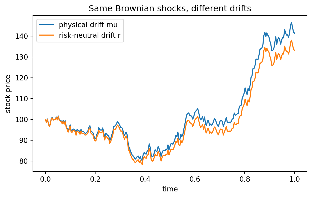
The physical measure uses drift $\mu$. The risk-neutral measure uses drift $r$. The volatility is the same in the Black--Scholes model.
```{python}
#| label: ch15-physical-risk-neutral-gbm
#| fig-cap: "Physical and risk-neutral GBM sample paths."
import numpy as np
import matplotlib.pyplot as plt

rng = np.random.default_rng(7243)

S0 = 100.0
mu = 0.10
r = 0.04
sigma = 0.25
T = 1.0
n = 252
dt = T / n

t = np.linspace(0, T, n + 1)
z = rng.normal(size=n)
W = np.concatenate([[0.0], np.cumsum(np.sqrt(dt) * z)])

S_physical = S0 * np.exp((mu - 0.5 * sigma**2) * t + sigma * W)
S_risk_neutral = S0 * np.exp((r - 0.5 * sigma**2) * t + sigma * W)

plt.figure(figsize=(7, 4))
plt.plot(t, S_physical, label="physical drift mu")
plt.plot(t, S_risk_neutral, label="risk-neutral drift r")
plt.xlabel("time")
plt.ylabel("stock price")
plt.title("Same Brownian shocks, different drifts")
plt.legend()
plt.show()
```
The same Brownian shocks can produce different expected growth depending on the measure. Pricing uses the risk-neutral dynamics, not the physical expected return.
## 15.15 Python Example: Discounted Stock as a Martingale Under $\mathbb Q$
Under the risk-neutral measure,
$$
dS_t=rS_t\,dt+\sigma S_t\,dW_t^{\mathbb Q}.
$$
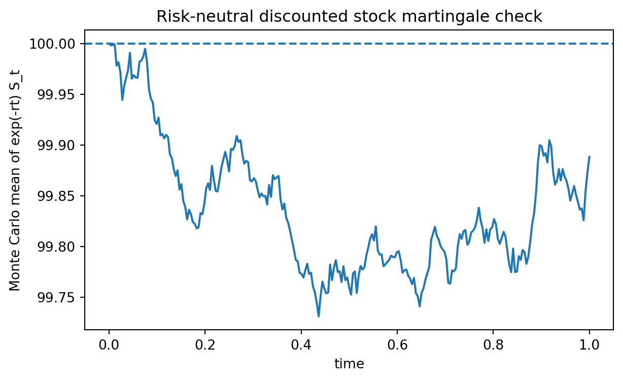
Therefore $e^{-rt}S_t$ should have constant expectation.
```{python}
#| label: ch15-discounted-stock-martingale
#| fig-cap: "The simulated mean of discounted risk-neutral stock prices is approximately constant."
import numpy as np
import matplotlib.pyplot as plt

rng = np.random.default_rng(5110)

S0 = 100.0
r = 0.04
sigma = 0.25
T = 1.0
n = 252
m = 20000
dt = T / n

t = np.linspace(0, T, n + 1)
Z = rng.normal(size=(m, n))
log_increments = (r - 0.5 * sigma**2) * dt + sigma * np.sqrt(dt) * Z
log_paths = np.cumsum(log_increments, axis=1)
S = np.concatenate([S0 * np.ones((m, 1)), S0 * np.exp(log_paths)], axis=1)

discounted_mean = np.mean(np.exp(-r * t) * S, axis=0)

plt.figure(figsize=(7, 4))
plt.plot(t, discounted_mean)
plt.axhline(S0, linestyle="--")
plt.xlabel("time")
plt.ylabel("Monte Carlo mean of exp(-rt) S_t")
plt.title("Risk-neutral discounted stock martingale check")
plt.show()

print("Initial value:", S0)
print("Final discounted mean:", discounted_mean[-1])
```
The final value will not equal $S_0$ exactly because of Monte Carlo error, but it should be close.
## 15.16 Python Example: Black--Scholes PDE Residual for Simple Claims
We can numerically check the residual
$$
R[V]=V_t+\frac12\sigma^2S^2V_{SS}+rSV_S-rV.
$$
```{python}
#| label: ch15-pde-residual-simple-claims
import numpy as np

r = 0.05
sigma = 0.30
K = 100.0
T = 1.0
t = 0.35
S = np.linspace(40, 160, 7)
tau = T - t

# Candidate 1: stock, V = S
V_stock = S
Vt_stock = np.zeros_like(S)
VS_stock = np.ones_like(S)
VSS_stock = np.zeros_like(S)
R_stock = Vt_stock + 0.5 * sigma**2 * S**2 * VSS_stock + r * S * VS_stock - r * V_stock

# Candidate 2: cash claim paying K at T, V = K exp(-r(T-t))
V_cash = K * np.exp(-r * tau) * np.ones_like(S)
Vt_cash = r * V_cash
VS_cash = np.zeros_like(S)
VSS_cash = np.zeros_like(S)
R_cash = Vt_cash + 0.5 * sigma**2 * S**2 * VSS_cash + r * S * VS_cash - r * V_cash

# Candidate 3: forward-style value, V = S - K exp(-r(T-t))
V_forward = S - K * np.exp(-r * tau)
Vt_forward = -r * K * np.exp(-r * tau) * np.ones_like(S)
VS_forward = np.ones_like(S)
VSS_forward = np.zeros_like(S)
R_forward = Vt_forward + 0.5 * sigma**2 * S**2 * VSS_forward + r * S * VS_forward - r * V_forward

print("stock residual:", np.round(R_stock, 12))
print("cash residual:", np.round(R_cash, 12))
print("forward residual:", np.round(R_forward, 12))
```
A residual close to zero means that the candidate is consistent with the Black--Scholes no-arbitrage equation.
## 15.17 Python Example: Monte Carlo Pricing Under $\mathbb Q$
For a European payoff $h(S_T)$, risk-neutral pricing gives
$$
V(0,S_0)=e^{-rT}\mathbb E^{\mathbb Q}[h(S_T)].
$$
For a call, $h(S_T)=(S_T-K)^+$. The closed-form formula is studied in Chapter 16. Here we use simulation to illustrate the risk-neutral expectation.
```{python}
#| label: ch15-risk-neutral-monte-carlo-call
import numpy as np

rng = np.random.default_rng(7339)

S0 = 100.0
K = 105.0
r = 0.04
sigma = 0.25
T = 1.0
m = 300000

Z = rng.normal(size=m)
ST = S0 * np.exp((r - 0.5 * sigma**2) * T + sigma * np.sqrt(T) * Z)
payoff = np.maximum(ST - K, 0.0)
price_mc = np.exp(-r * T) * payoff.mean()
standard_error = np.exp(-r * T) * payoff.std(ddof=1) / np.sqrt(m)

print("Monte Carlo call price:", price_mc)
print("Monte Carlo standard error:", standard_error)
print("Approximate 95% interval:", (price_mc - 1.96 * standard_error, price_mc + 1.96 * standard_error))
```
The simulation uses the risk-neutral drift $r$. Replacing $r$ by $\mu$ would estimate a physical expected discounted payoff, not the no-arbitrage price.
## 15.18 Python Example: Black--Scholes Formula Preview and PDE Check
Although Chapter 16 derives the closed-form formula, we can preview it and check the PDE numerically. For a call,
$$
C=S N(d_1)-Ke^{-r\tau}N(d_2),
$$
where $\tau=T-t$,
$$
d_1=\frac{\log(S/K)+(r+\frac12\sigma^2)\tau}{\sigma\sqrt\tau},
\qquad
d_2=d_1-\sigma\sqrt\tau.
$$
```{python}
#| label: ch15-call-formula-pde-check
import math
import numpy as np

def norm_cdf(x):
    return 0.5 * (1.0 + math.erf(x / math.sqrt(2.0)))

def bs_call(t, S, K, r, sigma, T):
    tau = T - t
    if tau <= 0:
        return max(S - K, 0.0)
    d1 = (math.log(S / K) + (r + 0.5 * sigma**2) * tau) / (sigma * math.sqrt(tau))
    d2 = d1 - sigma * math.sqrt(tau)
    return S * norm_cdf(d1) - K * math.exp(-r * tau) * norm_cdf(d2)

K = 100.0
r = 0.05
sigma = 0.25
T = 1.0
t = 0.4
S = 110.0

# finite-difference derivatives
h_t = 1e-4
h_s = 1e-2
V = bs_call(t, S, K, r, sigma, T)
Vt = (bs_call(t + h_t, S, K, r, sigma, T) - bs_call(t - h_t, S, K, r, sigma, T)) / (2 * h_t)
VS = (bs_call(t, S + h_s, K, r, sigma, T) - bs_call(t, S - h_s, K, r, sigma, T)) / (2 * h_s)
VSS = (bs_call(t, S + h_s, K, r, sigma, T) - 2 * V + bs_call(t, S - h_s, K, r, sigma, T)) / (h_s**2)

residual = Vt + 0.5 * sigma**2 * S**2 * VSS + r * S * VS - r * V

print("Call value:", V)
print("Delta approximation:", VS)
print("Gamma approximation:", VSS)
print("PDE residual:", residual)
```
The residual should be small relative to the option price. It is not exactly zero because we used numerical finite differences.
## 15.19 Python Example: Discrete Delta Hedging Error
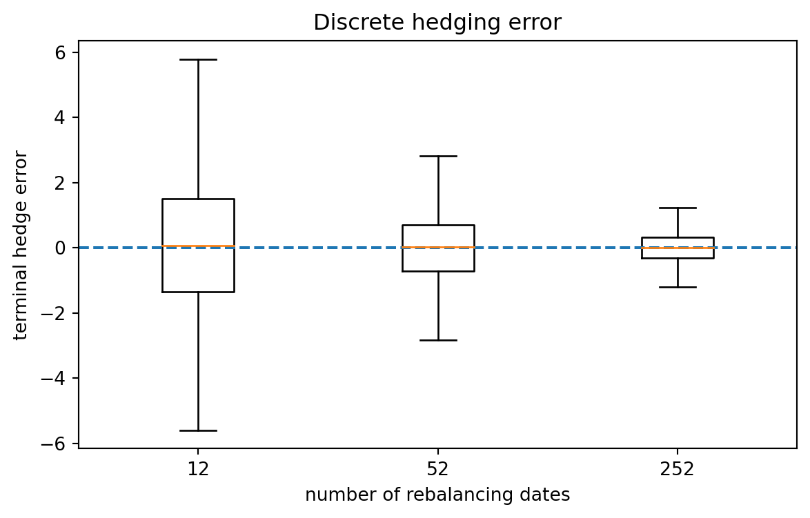
Exact replication requires continuous rebalancing. In practice, hedging is discrete. The next experiment simulates a short call hedged by Black--Scholes delta at a finite number of rebalancing dates.
```{python}
#| label: ch15-discrete-delta-hedging
#| fig-cap: "Discrete delta hedging error decreases as rebalancing becomes more frequent."
import math
import numpy as np
import matplotlib.pyplot as plt

rng = np.random.default_rng(2026)

def norm_cdf(x):
    return 0.5 * (1.0 + math.erf(x / math.sqrt(2.0)))

def bs_call_delta(t, S, K, r, sigma, T):
    tau = T - t
    if tau <= 0:
        return 1.0 if S > K else 0.0
    d1 = (math.log(S / K) + (r + 0.5 * sigma**2) * tau) / (sigma * math.sqrt(tau))
    return norm_cdf(d1)

def bs_call_price(t, S, K, r, sigma, T):
    tau = T - t
    if tau <= 0:
        return max(S - K, 0.0)
    d1 = (math.log(S / K) + (r + 0.5 * sigma**2) * tau) / (sigma * math.sqrt(tau))
    d2 = d1 - sigma * math.sqrt(tau)
    return S * norm_cdf(d1) - K * math.exp(-r * tau) * norm_cdf(d2)

def hedge_errors(n_steps, n_paths=5000):
    S0 = 100.0
    K = 100.0
    r = 0.03
    sigma = 0.25
    T = 1.0
    dt = T / n_steps
    errors = []
    for _ in range(n_paths):
        S = S0
        t = 0.0
        option0 = bs_call_price(t, S, K, r, sigma, T)
        delta = bs_call_delta(t, S, K, r, sigma, T)
        cash = option0 - delta * S
        for k in range(n_steps):
            z = rng.normal()
            S_new = S * math.exp((r - 0.5 * sigma**2) * dt + sigma * math.sqrt(dt) * z)
            cash *= math.exp(r * dt)
            t_new = (k + 1) * dt
            if k < n_steps - 1:
                new_delta = bs_call_delta(t_new, S_new, K, r, sigma, T)
                cash -= (new_delta - delta) * S_new
                delta = new_delta
            S = S_new
            t = t_new
        portfolio = delta * S + cash
        payoff = max(S - K, 0.0)
        errors.append(portfolio - payoff)
    return np.array(errors)

step_list = [12, 52, 252]
error_data = [hedge_errors(n) for n in step_list]

plt.figure(figsize=(7, 4))
plt.boxplot(error_data, labels=[str(n) for n in step_list], showfliers=False)
plt.axhline(0.0, linestyle="--")
plt.xlabel("number of rebalancing dates")
plt.ylabel("terminal hedge error")
plt.title("Discrete hedging error")
plt.show()

for n, e in zip(step_list, error_data):
    print(n, "steps: mean", e.mean(), "std", e.std(ddof=1))
```
The standard deviation of hedging error tends to shrink when the rebalancing frequency increases, although transaction costs and market frictions are not included here.
## 15.20 AI-Assisted Learning Components
::: {.callout-tip}
## AI prompt: Explain why $\mu$ cancels
Ask an AI tool:
> In the Black--Scholes delta hedging derivation, explain carefully why the physical drift $\mu$ cancels from the pricing PDE. Do not say only that we use risk-neutral probability. Show the cancellation from the Itô dynamics of $V(t,S_t)$ and the self-financing portfolio.
Then check whether the answer explicitly compares the $dt$ terms before and after choosing $\Delta=V_S$.
:::
::: {.callout-tip}
## AI prompt: Audit a self-financing argument
Ask an AI tool:
> A student writes $dX_t=\Delta_t dS_t+S_t d\Delta_t+\beta_t dB_t+B_t d\beta_t$ for a trading portfolio and concludes that the strategy is not self-financing unless $d\Delta_t=d\beta_t=0$. Identify the mistake and rewrite the self-financing condition correctly.
A good answer should explain that rebalancing can occur, but purchases of one asset must be financed by sales of the other.
:::
::: {.callout-tip}
## AI prompt: Check a simulation
Ask an AI tool:
> Review this Monte Carlo option-pricing code. Does it use the physical drift or the risk-neutral drift? Does the discount factor match the maturity? Does the payoff match the stated derivative?
This prompt is useful because many pricing-code errors are not syntax errors; they are modeling errors.
:::
## 15.21 Common Mistakes
1. **Using $\mu$ in the pricing expectation.** The expected stock return under the physical measure is not used in the risk-neutral pricing formula.
2. **Forgetting the Itô correction.** The $\frac12\sigma^2S^2V_{SS}$ term comes from quadratic variation.
3. **Confusing delta with probability.** Delta is a sensitivity, not the probability of finishing in the money.
4. **Ignoring self-financing.** A hedge must specify how rebalancing is paid for.
5. **Treating continuous hedging as realistic without qualification.** Real hedging is discrete and affected by costs, liquidity, and jumps.
6. **Forgetting the terminal condition.** The PDE must be solved backward from the payoff at maturity.
## 15.22 Exercises
### Conceptual exercises
1. Explain in your own words why no-arbitrage implies that a locally riskless portfolio must earn the risk-free rate.
2. Why does the Black--Scholes PDE contain $r$ and $\sigma$, but not $\mu$?
3. What does it mean for a trading strategy to be self-financing?
4. Why is $V_{SS}$ connected to the effect of randomness on the derivative price?
5. Explain the difference between a PDE derivation and a risk-neutral expectation formula.
### Mathematical exercises
6. Let $V(t,S)=S$. Verify directly that $V$ satisfies the Black--Scholes PDE.
7. Let $V(t,S)=Ke^{-r(T-t)}$. Verify directly that $V$ satisfies the PDE and has terminal value $K$.
8. Let $V(t,S)=S-Ke^{-r(T-t)}$. Interpret the associated replicating portfolio.
9. Starting from Itô's formula, derive the Black--Scholes PDE using the locally riskless portfolio $\Pi=V-V_SS$.
10. Suppose $V(t,S)=S^a e^{b(T-t)}$. Compute $R[V]$ and find the relation between $a$ and $b$ required for $V$ to solve the PDE.
### Computational exercises
11. Modify the Monte Carlo call-pricing code to price a put option.
12. Simulate risk-neutral stock paths and verify that $e^{-rt}S_t$ has approximately constant sample mean.
13. Use finite differences to estimate $V_t$, $V_S$, and $V_{SS}$ for a known formula and evaluate the PDE residual.
14. Repeat the delta-hedging experiment with different volatilities. How does hedging error change?
15. Repeat the delta-hedging experiment under physical drift $\mu\ne r$ while still hedging with Black--Scholes delta. Does the average hedging error change significantly?
### AI-assisted exercises
16. Ask an AI tool to derive the Black--Scholes PDE. Identify every assumption used in the derivation.
17. Ask an AI tool to explain the difference between $\mathbb P$ and $\mathbb Q$. Check whether it correctly states that they are probability measures on the same path space but with different drift dynamics.
18. Ask an AI tool to critique the Black--Scholes assumptions for modern markets. Separate mathematical limitations from empirical limitations.
19. Give an AI tool a deliberately incorrect PDE missing the gamma term. Ask it to find the error.
20. Ask an AI tool to propose tests for a delta-hedging simulation. Implement at least two of the tests in Python.
## 15.23 Chapter Summary
The Black--Scholes model is a continuous-time no-arbitrage model with one Brownian risk source and two traded assets: stock and cash. Because the market has exactly enough traded assets to hedge the Brownian risk, European derivatives can be replicated by self-financing strategies.
The mathematical steps are:
1. model the stock by GBM;
2. write the derivative value as $V(t,S_t)$;
3. apply Itô's formula;
4. choose the stock holding $\Delta=V_S$ to eliminate Brownian risk;
5. require the remaining locally riskless position to earn rate $r$;
6. obtain the Black--Scholes PDE;
7. solve backward from the terminal payoff.
The resulting PDE is
$$
V_t+\frac12\sigma^2S^2V_{SS}+rSV_S-rV=0.
$$
This equation is the bridge between stochastic calculus, dynamic hedging, partial differential equations, and risk-neutral pricing. Chapter 16 will solve this PDE for European call and put options and study the Greeks in detail.