import numpy as np
import pandas as pd
import matplotlib.pyplot as plt2 Introduction
Mathematical Finance as Modeling, Pricing, Hedging, and Risk Management
2.1 Why mathematical finance?
Financial markets provide a rich meeting place for probability, statistics, optimization, numerical analysis, and economic reasoning. A stock price, an option price, a bond yield, or a portfolio loss is not just a number. It is the output of a model, a set of assumptions, a calibration procedure, and a decision problem under uncertainty.
The purpose of this book is to develop the mathematical language needed to understand modern quantitative finance. The emphasis is not on memorizing formulas. The emphasis is on learning how to build models, derive prices, understand hedging, test assumptions, and measure risk.
A central theme is that the same mathematical object can have several complementary meanings.
| Object | Mathematical meaning | Financial meaning |
|---|---|---|
| Random variable | A measurable function | Future payoff, return, or loss |
| Conditional expectation | Best prediction under available information | Fair value under a pricing measure |
| Martingale | Process with no predictable drift | No-arbitrage discounted price process |
| Brownian motion | Continuous-time stochastic driver | Idealized source of market noise |
| PDE | Evolution equation for a value function | Option price as a function of state and time |
| Optimization problem | Maximize objective under constraints | Portfolio construction or calibration |
| Tail probability | Probability of extreme events | Market risk and capital requirement |
Mathematical finance is therefore both theoretical and computational. The theory explains why pricing formulas take their form. Computation shows how those formulas behave when assumptions are changed, when closed forms are unavailable, or when data are noisy.
2.2 Audience and prerequisites
This book is written for graduate students in applied mathematics, statistics, operations research, data science, and related quantitative fields. It may also be useful for advanced undergraduates with a strong mathematical background.
The expected preparation is:
- multivariable calculus and basic differential equations;
- linear algebra, especially vectors, matrices, inner products, and least squares;
- probability, including expectation, variance, conditional expectation, normal distributions, and limit theorems;
- basic statistics, including estimation, regression, and confidence intervals;
- some Python experience.
No previous finance background is required. The book introduces financial concepts as mathematical objects. For example, a bond is treated as a deterministic or stochastic cash-flow stream, an option is treated as a contingent payoff, and a portfolio is treated as a vector of weights applied to random returns.
NotePhilosophy of the book
The book is designed for readers who want to understand mathematical finance from first principles. Whenever possible, we begin with a small model, explain the mathematical structure, implement it in Python, and then discuss how the idea extends to more realistic settings.
2.3 The main questions
The book is organized around five recurring questions.
2.3.1 1. How do we model financial uncertainty?
We begin with discrete-time models of prices and returns. These models introduce no-arbitrage, self-financing portfolios, and risk-neutral probabilities. We then move to continuous-time models based on Brownian motion and stochastic differential equations.
Typical models include:
\[ S_{t+1}=S_t(1+R_{t+1}) \]
in discrete time and
\[ dS_t=\mu S_t\,dt+\sigma S_t\,dW_t \]
in continuous time. The first model emphasizes compounding and returns. The second model introduces geometric Brownian motion, the foundation of the Black–Scholes model.
2.3.2 2. How do we price contingent claims?
A contingent claim is a payoff that depends on uncertain future market variables. A European call option, for example, has payoff
\[ (S_T-K)^+. \]
In a no-arbitrage model, pricing is not simply about taking an expectation under the real-world probability measure. Instead, pricing uses a risk-neutral measure \(Q\) under which discounted tradable asset prices become martingales. The basic pricing formula is
\[ V_0=E^Q\left[e^{-rT}X\right], \]
where \(X\) is the payoff at maturity.
The book develops this idea first in binomial trees, then in Black–Scholes theory, Monte Carlo simulation, finite-difference methods, stochastic volatility models, and fixed-income models.
2.3.3 3. How do we hedge financial risk?
Pricing and hedging are deeply connected. In complete markets, the price of a derivative can be derived from a replicating portfolio. In the Black–Scholes model, the key hedge ratio is Delta:
\[ \Delta=\frac{\partial V}{\partial S}. \]
Dynamic Delta hedging illustrates both the power and the limitations of mathematical models. In ideal continuous time, perfect replication is possible under strong assumptions. In numerical experiments, hedging errors appear because trading is discrete, volatility may be misspecified, and real markets contain frictions.
2.3.4 4. How do we model interest rates and the yield curve?
Fixed-income markets require models for discount factors, zero rates, forward rates, and short rates. A zero-coupon bond price can be written as
\[ P(0,T)=e^{-T y(0,T)}, \]
where \(y(0,T)\) is the continuously compounded zero rate. In short-rate models, discounting depends on a stochastic process \(r_t\):
\[ P(t,T)=E^Q\left[\exp\left(-\int_t^T r_s\,ds\right)\mid \mathcal{F}_t\right]. \]
The book studies classical short-rate models such as Vasicek and CIR, and then introduces the Heath–Jarrow–Morton viewpoint, where the entire forward-rate curve evolves randomly.
2.3.5 5. How do we measure and manage risk?
A model is useful only if it helps us understand uncertainty and make decisions. The book studies portfolio optimization, factor models, Value at Risk, Expected Shortfall, stress testing, and model risk.
For a portfolio loss \(L\), Value at Risk at confidence level \(\alpha\) is a quantile:
\[ \operatorname{VaR}_\alpha(L)=\inf\{x:P(L\le x)\ge \alpha\}. \]
Expected Shortfall measures the average loss beyond the VaR threshold:
\[ \operatorname{ES}_\alpha(L)=E[L\mid L\ge \operatorname{VaR}_\alpha(L)]. \]
These quantities connect probability theory to practical risk management, but they also reveal the importance of distributional assumptions, dependence, tail behavior, and backtesting.
2.4 Computational approach
The computer labs are an essential part of the book. Each lab is written as a Google Colab notebook for independent study. Students should be able to open a notebook, read the background sections, run the code, modify parameters, and complete exercises without needing extra setup.
The labs use standard Python tools:
The computational style emphasizes:
- small models before large models;
- synthetic data before real data;
- transparent code before black-box libraries;
- numerical experiments that test mathematical claims;
- plots that reveal model behavior;
- exercises that ask students to change assumptions and interpret results.
TipHow to study with the labs
For each lab, first read the mathematical background without running code. Then run the notebook once from top to bottom. After that, change one parameter at a time and explain what changes mathematically and financially.
2.5 Roadmap of the labs
The labs form a computational spine for the book.
| Lab | Topic | Main mathematical idea |
|---|---|---|
| 1 | Prices, Returns, Compounding, and One-Period No-Arbitrage | Returns, portfolios, arbitrage |
| 2 | Multi-Period Binomial Trees and Risk-Neutral Pricing | Backward induction, replication |
| 3 | Brownian Motion, GBM, and Monte Carlo Pricing | Simulation, lognormal models |
| 4 | Black–Scholes Formula, Greeks, and Delta Hedging | PDE pricing, sensitivities |
| 5 | Implied Volatility and the Volatility Smile | Inverse problems, calibration |
| 6 | Monte Carlo Variance Reduction | Estimator variance, control variates |
| 7 | Exotic Options | Path dependence |
| 8 | Finite Difference Methods for the Black–Scholes PDE | Numerical PDEs |
| 9 | Ito Integrals and Ito Formula | Stochastic calculus by simulation |
| 10 | Martingales, Change of Measure, and Girsanov | Pricing measures |
| 11 | Interest Rates, Bonds, Duration, and Convexity | Discounting and sensitivity |
| 12 | Vasicek and CIR Short-Rate Models | Affine term-structure models |
| 13 | HJM and Yield-Curve Simulation | Forward-rate dynamics |
| 14 | Portfolio Optimization | Quadratic optimization |
| 15 | CAPM and Factor Models | Regression and risk decomposition |
| 16 | VaR, Expected Shortfall, and Backtesting | Tail risk and validation |
| 17 | Heston Stochastic Volatility | Volatility smiles and calibration |
| 18 | Integrated Pricing, Hedging, Calibration, and Risk | End-to-end quantitative workflow |
2.6 A first example: simple and log returns
Suppose a stock price moves from \(S_0\) to \(S_1\). The simple return is
\[ R=\frac{S_1-S_0}{S_0}, \]
while the log return is
\[ r=\log\left(\frac{S_1}{S_0}\right). \]
The two are related by
\[ r=\log(1+R), \qquad R=e^r-1. \]
For small returns, \(r\approx R\), but for larger moves the difference matters. Log returns are additive over time, while simple returns are directly connected to portfolio gains and losses.
import numpy as np
import matplotlib.pyplot as plt

R = np.linspace(-0.8, 1.0, 400)
r = np.log1p(R)

plt.figure(figsize=(7, 4))
plt.plot(R, r, label="log return log(1+R)")
plt.plot(R, R, linestyle="--", label="simple return R")
plt.xlabel("simple return R")
plt.ylabel("return scale")
plt.title("Simple return versus log return")
plt.legend()
plt.grid(True, alpha=0.3)
plt.show()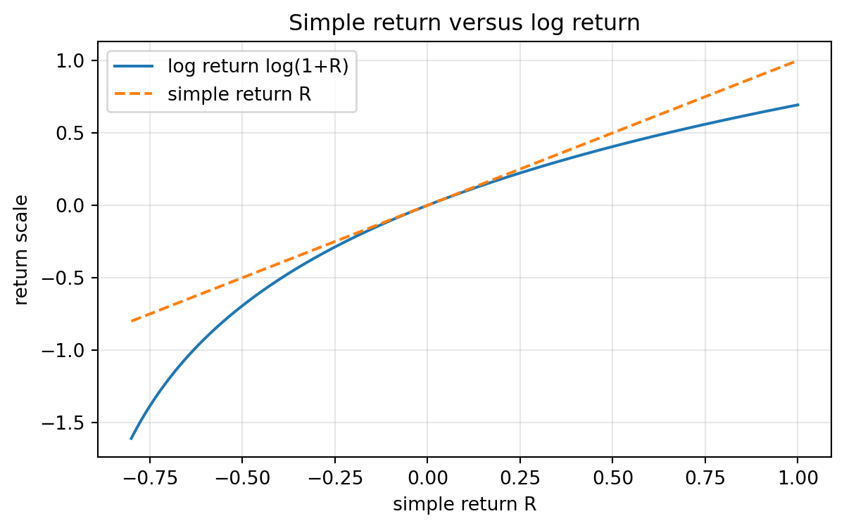
This small example illustrates the style of the book. A simple financial definition becomes a mathematical function. The function has properties. Those properties affect modeling choices. A short Python experiment then makes the difference visible.
2.7 Modeling assumptions and model risk
Every financial model is a simplification. The Black–Scholes model assumes continuous trading, constant volatility, no transaction costs, frictionless borrowing and lending, and lognormal stock prices. These assumptions are mathematically elegant, but they are not literally true.
The goal is not to find a perfect model. The goal is to understand what a model assumes, what it implies, how it can be computed, and where it may fail. This is why the book repeatedly compares:
- closed-form formulas and simulation;
- exact models and numerical approximations;
- model prices and market-implied quantities;
- ideal hedging and discrete hedging;
- normal risk models and heavy-tailed risk models.
A mathematically trained reader should become comfortable asking:
- What is the state variable?
- What is random and what is deterministic?
- Under which probability measure is the expectation taken?
- What is being calibrated?
- What is being hedged?
- What risk remains after hedging?
- Which assumptions are most important for the conclusion?
2.8 Suggested course use
A one-semester course can use this book in several ways.
2.8.1 Core mathematical finance path
A course focused on derivative pricing can emphasize:
- no-arbitrage and binomial models;
- Brownian motion and geometric Brownian motion;
- Black–Scholes theory;
- Greeks and hedging;
- Monte Carlo and finite differences;
- stochastic volatility.
2.8.2 Quantitative risk and portfolio path
A course focused on investment and risk can emphasize:
- returns and compounding;
- portfolio optimization;
- CAPM and factor models;
- VaR and Expected Shortfall;
- stress testing;
- integrated risk workflows.
2.8.3 Fixed-income path
A course with a fixed-income component can emphasize:
- bonds and yield curves;
- duration and convexity;
- short-rate models;
- HJM forward-rate modeling;
- interest-rate derivatives.
2.9 What students should be able to do
After working through the book and labs, students should be able to:
- explain no-arbitrage pricing in one-period and multi-period models;
- implement binomial-tree pricing and hedging algorithms;
- simulate Brownian motion and geometric Brownian motion;
- compute Black–Scholes prices and Greeks;
- estimate implied volatility from option prices;
- price path-dependent options by Monte Carlo;
- implement variance reduction methods;
- solve the Black–Scholes PDE numerically;
- explain Ito’s formula and change of measure at a computational level;
- price bonds from discount curves and analyze duration and convexity;
- simulate short-rate and forward-rate models;
- construct mean-variance portfolios under constraints;
- estimate CAPM and multi-factor models;
- compute and backtest VaR and Expected Shortfall;
- simulate and calibrate a basic stochastic-volatility model;
- combine pricing, hedging, calibration, and risk measurement in a complete workflow.
2.10 Final perspective
Mathematical finance is not only a collection of formulas. It is a way of translating uncertain future cash flows into mathematical objects that can be modeled, priced, hedged, optimized, and tested.
The central lesson of the book is that quantitative finance requires three kinds of understanding at the same time:
- Mathematical understanding: definitions, theorems, derivations, and assumptions.
- Computational understanding: algorithms, simulation, numerical approximation, and implementation.
- Financial understanding: interpretation, market meaning, hedging consequences, and risk limitations.
The reader should move back and forth among these three perspectives throughout the book. That movement is the real practice of mathematical finance.