---
title: "Chapter 11. Stochastic Integration"
---
::: {.chapter-objectives}
## Learning Goals
By the end of this chapter, students should be able to:
- explain why ordinary Riemann integration is not sufficient for Brownian-driven models;
- define simple predictable processes and the Itô integral first for simple integrands;
- extend the Itô integral by the Itô isometry;
- distinguish adapted, predictable, and anticipative integrands;
- compute basic stochastic integrals such as $\int_0^T f(t)\,dW_t$ and $\int_0^T W_t\,dW_t$;
- prove the martingale property and second-moment formula for Itô integrals;
- explain how quadratic variation changes the rules of calculus;
- connect stochastic integration with self-financing trading strategies;
- simulate stochastic integrals in Python using left-endpoint sums;
- use AI tools to audit stochastic-integral simulations and identify invalid uses of future information.
:::
::: {.hero-box}
Brownian motion is too irregular for ordinary differential calculus. Its paths are continuous, but they have infinite total variation and nonzero quadratic variation. Therefore, an expression such as
$$
\int_0^T H_t\,dW_t
$$
cannot be interpreted as an ordinary Riemann--Stieltjes integral for most useful integrands $H_t$.
The Itô integral is the stochastic integral designed for finance. It uses **only information available before the Brownian increment occurs**. This left-endpoint convention is the mathematical expression of a trading rule that cannot look into the future.
:::
## 11.1 Why a New Integral Is Needed
In ordinary calculus, the integral
$$
\int_0^T h(t)\,dx(t)
$$
can often be defined when $x(t)$ has bounded variation. A continuous function $x$ has bounded variation on $[0,T]$ if
$$
\sup_{\Pi}\sum_{i=0}^{n-1}|x(t_{i+1})-x(t_i)| < \infty,
$$
where the supremum is over all partitions
$$
0=t_0<t_1<\cdots<t_n=T.
$$
Brownian motion does not have bounded variation. In fact, for Brownian motion,
$$
\sum_i |W_{t_{i+1}}-W_{t_i}|
$$
usually grows without bound as the mesh of the partition goes to zero. But the squared increments have a stable limit:
$$
\sum_i (W_{t_{i+1}}-W_{t_i})^2 \to T.
$$
This is the quadratic variation relation
$$
[W]_T=T.
$$
The existence of quadratic variation is the reason the stochastic calculus of Brownian motion differs from ordinary calculus.
::: {.remark}
A useful informal rule is
$$
\Delta W \text{ has size about } \sqrt{\Delta t}.
$$
Therefore
$$
(\Delta W)^2 \text{ has size about } \Delta t.
$$
This explains why second-order terms survive in stochastic calculus.
:::
## 11.2 Financial Motivation: Trading Gains
Suppose $S_t$ is a risky asset price and $H_t$ is the number of shares held at time $t$. The cumulative trading gain should be written as
$$
\int_0^T H_t\,dS_t.
$$
In discrete time, if trading dates are
$$
0=t_0<t_1<\cdots<t_n=T,
$$
then the gain from trading is
$$
\sum_{i=0}^{n-1} H_{t_i}(S_{t_{i+1}}-S_{t_i}).
$$
The key feature is that $H_{t_i}$ is chosen at time $t_i$, before the price increment $S_{t_{i+1}}-S_{t_i}$ is known. The continuous-time stochastic integral preserves exactly this logic:
$$
\int_0^T H_t\,dS_t
\approx
\sum_{i=0}^{n-1} H_{t_i}(S_{t_{i+1}}-S_{t_i}).
$$
For Brownian-driven models, this left-endpoint construction gives the Itô integral.
::: {.callout-note}
## Finance interpretation
The Itô integral is not just a technical construction. It encodes the no-foresight condition of a trading strategy. If the integrand were allowed to depend on future increments, the model could accidentally permit unrealistic trading gains.
:::
## 11.3 Information, Adaptedness, and Predictability
Let $(\Omega,\mathcal F,\mathbb P)$ be a probability space and let $(\mathcal F_t)_{t\ge 0}$ be a filtration. The sigma-algebra $\mathcal F_t$ represents the information available up to time $t$.
::: {.definition}
### Definition 11.1: Adapted process
A stochastic process $(H_t)_{t\ge 0}$ is adapted to the filtration $(\mathcal F_t)_{t\ge 0}$ if $H_t$ is $\mathcal F_t$-measurable for every $t$.
:::
Adaptedness says that the value of $H_t$ can be determined from information available at time $t$. In finance, this means the portfolio position at time $t$ is based only on current and past information.
For the construction of the Itô integral, the most transparent starting point is a simple process of the form
$$
H_t=\sum_{i=0}^{n-1} H_i\mathbf 1_{(t_i,t_{i+1}]}(t),
$$
where $H_i$ is $\mathcal F_{t_i}$-measurable. This means that the value used on the interval $(t_i,t_{i+1}]$ is known at the left endpoint $t_i$.
::: {.definition}
### Definition 11.2: Simple predictable process
A process $H$ is a simple predictable process on $[0,T]$ if there is a partition
$$
0=t_0<t_1<\cdots<t_n=T
$$
such that
$$
H_t=\sum_{i=0}^{n-1} H_i\mathbf 1_{(t_i,t_{i+1}]}(t),
$$
where each $H_i$ is bounded and $\mathcal F_{t_i}$-measurable.
:::
The word predictable means that the integrand is fixed before the next Brownian increment is observed.
## 11.4 The Itô Integral for Simple Processes
Let $W_t$ be Brownian motion adapted to $(\mathcal F_t)$. For a simple predictable process
$$
H_t=\sum_{i=0}^{n-1} H_i\mathbf 1_{(t_i,t_{i+1}]}(t),
$$
the Itô integral is defined by
$$
\int_0^T H_t\,dW_t
=
\sum_{i=0}^{n-1} H_i(W_{t_{i+1}}-W_{t_i}).
$$
This is the stochastic counterpart of a left-endpoint Riemann sum.
::: {.example}
### Example 11.1: Constant integrand
If $H_t=c$, then
$$
\int_0^T c\,dW_t
=
\sum_{i=0}^{n-1} c(W_{t_{i+1}}-W_{t_i})
=c(W_T-W_0)
=cW_T.
$$
Therefore
$$
\int_0^T c\,dW_t \sim N(0,c^2T).
$$
:::
::: {.example}
### Example 11.2: One-step random integrand
Let
$$
H_t=H_0\mathbf 1_{(0,T]}(t),
$$
where $H_0$ is $\mathcal F_0$-measurable and bounded. Then
$$
\int_0^T H_t\,dW_t=H_0W_T.
$$
If $H_0$ is deterministic, this is normal. If $H_0$ is random, the integral is conditionally normal given $H_0$.
:::
## 11.5 Mean and Variance of a Simple Itô Integral
For a simple predictable process,
$$
I_T=\int_0^T H_t\,dW_t
=
\sum_{i=0}^{n-1} H_i\Delta W_i,
$$
where
$$
\Delta W_i=W_{t_{i+1}}-W_{t_i}.
$$
Because $H_i$ is $\mathcal F_{t_i}$-measurable and $\Delta W_i$ is independent of $\mathcal F_{t_i}$ with mean zero,
$$
\mathbb E[H_i\Delta W_i]=0.
$$
Thus
$$
\mathbb E[I_T]=0.
$$
For the second moment, cross terms vanish. Therefore
$$
\mathbb E[I_T^2]
=
\sum_{i=0}^{n-1}\mathbb E[H_i^2(\Delta W_i)^2]
=
\sum_{i=0}^{n-1}\mathbb E[H_i^2](t_{i+1}-t_i).
$$
This is
$$
\mathbb E\left[\left(\int_0^T H_t\,dW_t\right)^2\right]
=
\mathbb E\left[\int_0^T H_t^2\,dt\right].
$$
This identity is called the Itô isometry.
::: {.theorem}
### Theorem 11.1: Itô isometry for simple predictable processes
If $H$ is a simple predictable process on $[0,T]$, then
$$
\mathbb E\left[\int_0^T H_t\,dW_t\right]=0
$$
and
$$
\mathbb E\left[\left(\int_0^T H_t\,dW_t\right)^2\right]
=
\mathbb E\left[\int_0^T H_t^2\,dt\right].
$$
:::
::: {.proof}
Write $I_T=\sum_i H_i\Delta W_i$. Since $H_i$ is known at time $t_i$ and $\Delta W_i$ is independent of $\mathcal F_{t_i}$ with mean zero,
$$
\mathbb E[H_i\Delta W_i]
=\mathbb E[H_i\mathbb E[\Delta W_i\mid \mathcal F_{t_i}]]=0.
$$
For the second moment,
$$
\mathbb E[I_T^2]
=
\sum_i\mathbb E[H_i^2(\Delta W_i)^2]
+2\sum_{i<j}\mathbb E[H_iH_j\Delta W_i\Delta W_j].
$$
The cross terms are zero by conditioning on the earlier information before the later increment. Also,
$$
\mathbb E[(\Delta W_i)^2\mid \mathcal F_{t_i}]=t_{i+1}-t_i.
$$
Hence
$$
\mathbb E[I_T^2]
=
\sum_i\mathbb E[H_i^2](t_{i+1}-t_i)
=\mathbb E\left[\int_0^T H_t^2\,dt\right].
$$
:::
## 11.6 Extension by Completion in $L^2$
The simple-process definition is not enough for applications. We want to integrate processes such as $H_t=W_t$, $H_t=S_t$, or $H_t=\sigma(t,S_t)$. The Itô isometry gives the correct extension.
Let $\mathcal H^2[0,T]$ denote the space of adapted processes satisfying
$$
\mathbb E\left[\int_0^T H_t^2\,dt\right]<\infty.
$$
For $H\in\mathcal H^2[0,T]$, choose simple predictable processes $H^{(n)}$ such that
$$
\mathbb E\left[\int_0^T (H_t^{(n)}-H_t)^2\,dt\right]\to 0.
$$
Then define
$$
\int_0^T H_t\,dW_t
=
\lim_{n\to\infty}\int_0^T H_t^{(n)}\,dW_t
$$
where the limit is in $L^2(\Omega)$.
The Itô isometry guarantees that this limit is well-defined and independent of the approximating sequence.
::: {.theorem}
### Theorem 11.2: Itô isometry
If $H\in\mathcal H^2[0,T]$, then the Itô integral $\int_0^T H_t\,dW_t$ is well-defined in $L^2$ and satisfies
$$
\mathbb E\left[\int_0^T H_t\,dW_t\right]=0,
$$
$$
\mathbb E\left[\left(\int_0^T H_t\,dW_t\right)^2\right]
=
\mathbb E\left[\int_0^T H_t^2\,dt\right].
$$
:::
## 11.7 The Itô Integral as a Martingale
For $0\le t\le T$, define
$$
M_t=\int_0^t H_s\,dW_s.
$$
Under square-integrability assumptions, $(M_t)$ is a martingale.
::: {.theorem}
### Theorem 11.3: Martingale property
If $H\in\mathcal H^2[0,T]$, then
$$
M_t=\int_0^t H_s\,dW_s
$$
is an $L^2$ martingale with respect to $(\mathcal F_t)$. That is, for $0\le s\le t\le T$,
$$
\mathbb E[M_t\mid \mathcal F_s]=M_s.
$$
:::
The martingale property comes from the fact that future Brownian increments have conditional mean zero and are independent of current information.
This theorem is central in finance. Under a risk-neutral measure, the stochastic part of a discounted asset price is often written as an Itô integral, and therefore has no predictable drift.
## 11.8 Deterministic Integrands
If $f:[0,T]\to\mathbb R$ is deterministic and square-integrable, then
$$
I_T=\int_0^T f(t)\,dW_t
$$
is normally distributed with mean zero and variance
$$
\int_0^T f(t)^2\,dt.
$$
Hence
$$
\int_0^T f(t)\,dW_t
\sim
N\left(0,\int_0^T f(t)^2\,dt\right).
$$
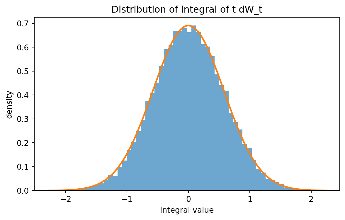
::: {.example}
### Example 11.3: Integrating $t$ against Brownian motion
Let $f(t)=t$. Then
$$
\int_0^T t\,dW_t
\sim
N\left(0,\int_0^T t^2\,dt\right)
=
N\left(0,\frac{T^3}{3}\right).
$$
:::
```{python}
#| label: py-ch11-deterministic-integrand
#| fig-cap: "Monte Carlo distribution of an Itô integral with deterministic integrand."
import numpy as np
import matplotlib.pyplot as plt

rng = np.random.default_rng(7243)
T = 1.0
n = 1000
m = 20000
dt = T / n

t = np.linspace(0, T, n + 1)
left_t = t[:-1]
f = left_t

dW = rng.normal(0.0, np.sqrt(dt), size=(m, n))
I = dW @ f

theory_var = T**3 / 3
print("Monte Carlo mean:", I.mean())
print("Monte Carlo variance:", I.var(ddof=1))
print("Theoretical variance:", theory_var)

plt.figure(figsize=(7, 4))
plt.hist(I, bins=60, density=True, alpha=0.65)
x = np.linspace(I.min(), I.max(), 400)
density = (1 / np.sqrt(2 * np.pi * theory_var)) * np.exp(-x**2 / (2 * theory_var))
plt.plot(x, density, linewidth=2)
plt.xlabel("integral value")
plt.ylabel("density")
plt.title("Distribution of integral of t dW_t")
plt.show()
```
## 11.9 The Integral $\int_0^T W_t\,dW_t$
One of the most important examples is
$$
\int_0^T W_t\,dW_t.
$$
The Itô integral is computed using left endpoints:
$$
\int_0^T W_t\,dW_t
=\lim_{|\Pi|\to 0}\sum_{i=0}^{n-1}W_{t_i}(W_{t_{i+1}}-W_{t_i}).
$$
Using the algebraic identity
$$
W_{t_{i+1}}^2-W_{t_i}^2
=2W_{t_i}\Delta W_i+(\Delta W_i)^2,
$$
we get
$$
W_{t_i}\Delta W_i
=\frac12(W_{t_{i+1}}^2-W_{t_i}^2)-\frac12(\Delta W_i)^2.
$$
Summing over $i$ gives
$$
\sum_i W_{t_i}\Delta W_i
=\frac12 W_T^2-\frac12\sum_i(\Delta W_i)^2.
$$
Since
$$
\sum_i(\Delta W_i)^2\to T,
$$
we obtain
$$
\int_0^T W_t\,dW_t
=�rac12(W_T^2-T).
$$
::: {.warning}
In ordinary calculus, one might guess
$$
\int_0^T W_t\,dW_t=\frac12W_T^2.
$$
This is wrong for the Itô integral. The missing correction is $-T/2$, coming from quadratic variation.
:::
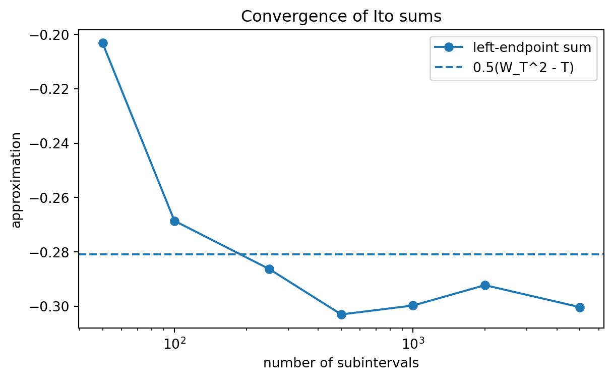
```{python}
#| label: py-ch11-w-dw-one-path
#| fig-cap: "Left-endpoint sums approximate the Itô integral of W_t dW_t."
import numpy as np
import matplotlib.pyplot as plt

rng = np.random.default_rng(7339)
T = 1.0
n_fine = 20000
dt = T / n_fine

dW = rng.normal(0.0, np.sqrt(dt), size=n_fine)
W = np.concatenate([[0.0], np.cumsum(dW)])

levels = [50, 100, 250, 500, 1000, 2000, 5000]
approx = []
for n in levels:
    step = n_fine // n
    idx = np.arange(0, n_fine + 1, step)
    idx[-1] = n_fine
    Wc = W[idx]
    dWc = np.diff(Wc)
    approx.append(np.sum(Wc[:-1] * dWc))

theory = 0.5 * (W[-1]**2 - T)
print("Theoretical value from Ito formula:", theory)
for n, val in zip(levels, approx):
    print(f"n={n:5d}: left sum = {val:.6f}")

plt.figure(figsize=(7, 4))
plt.plot(levels, approx, marker="o", label="left-endpoint sum")
plt.axhline(theory, linestyle="--", label="0.5(W_T^2 - T)")
plt.xscale("log")
plt.xlabel("number of subintervals")
plt.ylabel("approximation")
plt.title("Convergence of Ito sums")
plt.legend()
plt.show()
```
## 11.10 Itô Versus Stratonovich Sums
The choice of evaluation point matters. For Brownian motion, compare three sums:
$$
\sum_i W_{t_i}\Delta W_i,
$$
$$
\sum_i \frac{W_{t_i}+W_{t_{i+1}}}{2}\Delta W_i,
$$
and
$$
\sum_i W_{t_{i+1}}\Delta W_i.
$$
The first is the Itô left-endpoint sum. The second is the midpoint or Stratonovich-style sum. The third is a right-endpoint sum that uses future information.
For the integral of $W_t$ against $W_t$, the limiting values are
$$
\text{Itô:}\quad \frac12(W_T^2-T),
$$
$$
\text{Stratonovich:}\quad \frac12W_T^2,
$$
$$
\text{right endpoint:}\quad \frac12(W_T^2+T).
$$
The financial convention is the Itô convention because trading positions are chosen before the next price movement is observed.
## 11.11 Interactive: Itô, Midpoint, and Right-Endpoint Sums
Move the slider to change the number of subintervals used to approximate $\int_0^T W_t\,dW_t$ on the same Brownian path. The left, midpoint, and right sums approach different limits.
::: {.interactive-card}
<div class="mf-controls">
<label for="ch11-nsum">number of subintervals</label>
<span id="ch11-nsum-val">200</span>
<input id="ch11-nsum" type="range" min="20" max="1200" step="20" value="200">
<span></span>
</div>
<div id="ch11-ito-sums-demo" class="plotly-demo"></div>
<div id="ch11-ito-sums-output" class="mf-output"></div>
:::
<script>
(window.mfPlotlyReady || function(f){ if (document.readyState === "loading") { document.addEventListener("DOMContentLoaded", f); } else { f(); } })(function() {
var plot = document.getElementById("ch11-ito-sums-demo");
if (!plot || typeof Plotly === "undefined") return;
var slider = document.getElementById("ch11-nsum");
var sliderVal = document.getElementById("ch11-nsum-val");
var output = document.getElementById("ch11-ito-sums-output");
function normalRandom() {
var u = 0, v = 0;
while (u === 0) u = Math.random();
while (v === 0) v = Math.random();
return Math.sqrt(-2.0 * Math.log(u)) * Math.cos(2.0 * Math.PI * v);
}
var T = 1.0;
var nFine = 6000;
var dt = T / nFine;
var tFine = new Array(nFine + 1);
var wFine = new Array(nFine + 1);
tFine[0] = 0;
wFine[0] = 0;
for (var i = 1; i <= nFine; i++) {
tFine[i] = i * dt;
wFine[i] = wFine[i - 1] + Math.sqrt(dt) * normalRandom();
}
function compute(n) {
var step = Math.max(1, Math.floor(nFine / n));
var idx = [];
for (var i = 0; i < nFine; i += step) idx.push(i);
if (idx[idx.length - 1] !== nFine) idx.push(nFine);
var x = [];
var y = [];
var left = 0, mid = 0, right = 0, qv = 0;
for (var k = 0; k < idx.length; k++) {
x.push(tFine[idx[k]]);
y.push(wFine[idx[k]]);
}
for (var k = 0; k < idx.length - 1; k++) {
var a = wFine[idx[k]];
var b = wFine[idx[k + 1]];
var dw = b - a;
left += a * dw;
mid += 0.5 * (a + b) * dw;
right += b * dw;
qv += dw * dw;
}
return {x: x, y: y, left: left, mid: mid, right: right, qv: qv};
}
function update() {
var n = parseInt(slider.value, 10);
sliderVal.textContent = n.toString();
var result = compute(n);
var WT = wFine[nFine];
var itoLimit = 0.5 * (WT * WT - T);
var stratLimit = 0.5 * WT * WT;
var rightLimit = 0.5 * (WT * WT + T);
var traces = [
{x: result.x, y: result.y, mode: "lines", name: "Brownian path"},
{x: [0, T], y: [0, 0], mode: "lines", name: "zero line", line: {dash: "dot"}}
];
var layout = {
title: "One Brownian path used for stochastic sums",
xaxis: {title: "time"},
yaxis: {title: "W(t)"},
margin: {l: 55, r: 20, t: 50, b: 50}
};
Plotly.react(plot, traces, layout, {responsive: true});
output.innerHTML = "left sum = " + result.left.toFixed(4) +
", midpoint sum = " + result.mid.toFixed(4) +
", right sum = " + result.right.toFixed(4) +
", quadratic variation sum = " + result.qv.toFixed(4) +
"<br>theoretical Ito limit = " + itoLimit.toFixed(4) +
", midpoint limit = " + stratLimit.toFixed(4) +
", right-endpoint limit = " + rightLimit.toFixed(4);
}
slider.addEventListener("input", update);
update();
});
</script>
## 11.12 Interactive: Itô Isometry for Deterministic Integrands
For a deterministic function $f$, the integral $\int_0^T f(t)\,dW_t$ is normal with variance $\int_0^T f(t)^2\,dt$. This interactive simulation uses
$$
f(t)=a+b\sin(2\pi t).
$$
::: {.interactive-card}
<div class="mf-controls">
<label for="ch11-a">constant level $a$</label>
<span id="ch11-a-val">1.00</span>
<input id="ch11-a" type="range" min="-2" max="2" step="0.05" value="1">
<span></span>
<label for="ch11-b">oscillation size $b$</label>
<span id="ch11-b-val">0.80</span>
<input id="ch11-b" type="range" min="0" max="2" step="0.05" value="0.8">
<span></span>
</div>
<div id="ch11-isometry-demo" class="plotly-demo"></div>
<div id="ch11-isometry-output" class="mf-output"></div>
:::
<script>
(window.mfPlotlyReady || function(f){ if (document.readyState === "loading") { document.addEventListener("DOMContentLoaded", f); } else { f(); } })(function() {
var plot = document.getElementById("ch11-isometry-demo");
if (!plot || typeof Plotly === "undefined") return;
var aSlider = document.getElementById("ch11-a");
var bSlider = document.getElementById("ch11-b");
var aVal = document.getElementById("ch11-a-val");
var bVal = document.getElementById("ch11-b-val");
var output = document.getElementById("ch11-isometry-output");
function normalRandom() {
var u = 0, v = 0;
while (u === 0) u = Math.random();
while (v === 0) v = Math.random();
return Math.sqrt(-2.0 * Math.log(u)) * Math.cos(2.0 * Math.PI * v);
}
function normalDensity(x, variance) {
return Math.exp(-0.5 * x * x / variance) / Math.sqrt(2 * Math.PI * variance);
}
function update() {
var a = parseFloat(aSlider.value);
var b = parseFloat(bSlider.value);
aVal.textContent = a.toFixed(2);
bVal.textContent = b.toFixed(2);
var T = 1.0;
var n = 300;
var m = 1600;
var dt = T / n;
var samples = [];
var variance = 0;
for (var i = 0; i < n; i++) {
var t = i * dt;
var f = a + b * Math.sin(2 * Math.PI * t);
variance += f * f * dt;
}
for (var j = 0; j < m; j++) {
var total = 0;
for (var i = 0; i < n; i++) {
var t = i * dt;
var f = a + b * Math.sin(2 * Math.PI * t);
total += f * Math.sqrt(dt) * normalRandom();
}
samples.push(total);
}
var sd = Math.sqrt(variance);
var xs = [];
var ys = [];
var minX = -4 * Math.max(sd, 0.1);
var maxX = 4 * Math.max(sd, 0.1);
for (var k = 0; k < 200; k++) {
var x = minX + (maxX - minX) * k / 199;
xs.push(x);
ys.push(normalDensity(x, variance));
}
var traces = [
{x: samples, type: "histogram", histnorm: "probability density", nbinsx: 40, name: "simulated integrals"},
{x: xs, y: ys, mode: "lines", name: "normal density from Ito isometry"}
];
var layout = {
title: "Distribution of integral of f(t) dW_t",
xaxis: {title: "integral value"},
yaxis: {title: "density"},
bargap: 0.04,
margin: {l: 55, r: 20, t: 50, b: 50}
};
Plotly.react(plot, traces, layout, {responsive: true});
var sampleMean = samples.reduce(function(s, v) { return s + v; }, 0) / samples.length;
var sampleVar = samples.reduce(function(s, v) { return s + (v - sampleMean) * (v - sampleMean); }, 0) / (samples.length - 1);
output.innerHTML = "theoretical variance = " + variance.toFixed(4) +
", simulated variance = " + sampleVar.toFixed(4) +
", simulated mean = " + sampleMean.toFixed(4);
}
aSlider.addEventListener("input", update);
bSlider.addEventListener("input", update);
update();
});
</script>
## 11.13 Quadratic Variation and the Differential Rules
The Itô integral is deeply connected to quadratic variation. In formal stochastic differential notation, the central rules are
$$
dt\,dt=0,
$$
$$
dt\,dW_t=0,
$$
$$
dW_t\,dW_t=dt.
$$
These are not ordinary multiplication rules. They encode the limiting size of Brownian increments.
If
$$
dX_t=\mu_t\,dt+\sigma_t\,dW_t,
$$
then the quadratic variation contribution comes only from the Brownian part:
$$
(dX_t)^2=\sigma_t^2\,dt.
$$
This rule is the foundation of Itô's formula in the next chapter.
## 11.14 Stochastic Integrals with Respect to Itô Processes
An Itô process has the form
$$
X_t=X_0+\int_0^t \mu_s\,ds+\int_0^t \sigma_s\,dW_s.
$$
Equivalently, we write
$$
dX_t=\mu_t\,dt+\sigma_t\,dW_t.
$$
If $H_t$ is an admissible integrand, then
$$
\int_0^T H_t\,dX_t
=
\int_0^T H_t\mu_t\,dt+
\int_0^T H_t\sigma_t\,dW_t.
$$
The first integral is an ordinary time integral. The second is an Itô integral.
::: {.example}
### Example 11.4: Trading gain in an arithmetic Brownian model
Suppose
$$
dS_t=\mu\,dt+\sigma\,dW_t.
$$
If a strategy holds $H_t$ shares, then the gain is
$$
\int_0^T H_t\,dS_t
=
\int_0^T H_t\mu\,dt+
\int_0^T H_t\sigma\,dW_t.
$$
The first part is predictable drift exposure. The second part is random Brownian exposure.
:::
## 11.15 Self-Financing Strategies in Continuous Time
Let $B_t$ be a riskless asset and $S_t$ a risky asset. A portfolio has value
$$
V_t=\phi_t B_t+\Delta_t S_t,
$$
where $\phi_t$ is the number of units of the riskless asset and $\Delta_t$ is the number of shares of the risky asset.
The strategy is self-financing if changes in wealth are caused only by gains and losses on the assets, not by adding or withdrawing external cash:
$$
dV_t=\phi_t\,dB_t+\Delta_t\,dS_t.
$$
This formula is a stochastic-integral statement. In integral form,
$$
V_T=V_0+\int_0^T \phi_t\,dB_t+\int_0^T \Delta_t\,dS_t.
$$
The integrand $\Delta_t$ must be nonanticipative. A hedging strategy cannot depend on tomorrow's Brownian increment.
::: {.warning}
A common mistake is to differentiate the identity $V_t=\phi_tB_t+\Delta_tS_t$ using an ordinary product rule and then include extra terms such as $B_t\,d\phi_t$ and $S_t\,d\Delta_t$ in the self-financing condition. Those terms are financed internally by rebalancing. The self-financing condition defines the wealth dynamics directly as gains from held assets.
:::
## 11.16 Why Anticipation Is Dangerous
Consider a discrete approximation to the Brownian integral. The valid Itô sum uses
$$
\sum_i H_{t_i}\Delta W_i.
$$
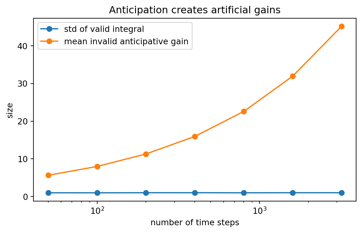
If one were allowed to choose
$$
H_{t_i}=\operatorname{sign}(\Delta W_i),
$$
then the sum becomes
$$
\sum_i |\Delta W_i|,
$$
which grows very large as the partition becomes fine. This would create unrealistic profits from knowing the next increment before it occurs.
This example explains why adaptedness and predictability are not optional technical details. They are mathematical forms of the no-foresight principle.
```{python}
#| label: py-ch11-anticipating-strategy
#| fig-cap: "An invalid anticipative strategy creates artificial gains."
import numpy as np
import matplotlib.pyplot as plt

rng = np.random.default_rng(2026)
T = 1.0
levels = np.array([50, 100, 200, 400, 800, 1600, 3200])
m = 5000

valid_std = []
anticipating_mean = []
for n in levels:
    dt = T / n
    dW = rng.normal(0.0, np.sqrt(dt), size=(m, n))
    valid = dW.sum(axis=1)                 # H_i = 1
    anticipating = np.abs(dW).sum(axis=1)  # H_i = sign(dW_i), not admissible
    valid_std.append(valid.std(ddof=1))
    anticipating_mean.append(anticipating.mean())

plt.figure(figsize=(7, 4))
plt.plot(levels, valid_std, marker="o", label="std of valid integral")
plt.plot(levels, anticipating_mean, marker="o", label="mean invalid anticipative gain")
plt.xscale("log")
plt.xlabel("number of time steps")
plt.ylabel("size")
plt.title("Anticipation creates artificial gains")
plt.legend()
plt.show()
```
## 11.17 Simulation of Itô Integrals
For practical computation, an Itô integral is approximated by
$$
\int_0^T H_t\,dW_t
\approx
\sum_{i=0}^{n-1}H_{t_i}\Delta W_i.
$$
The left endpoint is essential. A reliable simulation procedure is:
1. Choose a time grid.
2. Simulate Brownian increments $\Delta W_i\sim N(0,\Delta t)$.
3. Build the adapted process $H_{t_i}$ using information up to time $t_i$.
4. Sum $H_{t_i}\Delta W_i$.
5. Repeat many times to estimate the distribution.
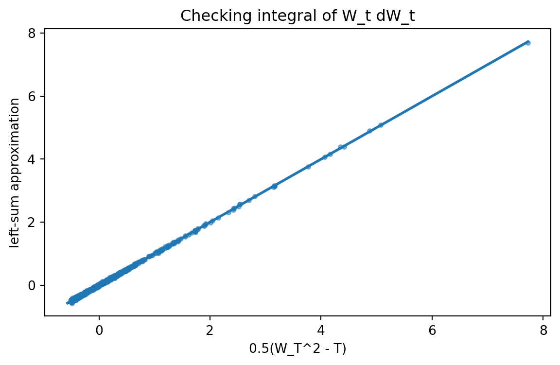
```{python}
#| label: py-ch11-simulate-H-W
#| fig-cap: "Monte Carlo simulation of integral of W_t dW_t."
import numpy as np
import matplotlib.pyplot as plt

rng = np.random.default_rng(5110)
T = 1.0
n = 1200
m = 20000
dt = T / n

dW = rng.normal(0.0, np.sqrt(dt), size=(m, n))
W_left = np.concatenate([np.zeros((m, 1)), np.cumsum(dW, axis=1)[:, :-1]], axis=1)
I = np.sum(W_left * dW, axis=1)
W_T = np.sum(dW, axis=1)
theory = 0.5 * (W_T**2 - T)

print("Mean of Ito sum:", I.mean())
print("Variance of Ito sum:", I.var(ddof=1))
print("Mean absolute difference from formula:", np.mean(np.abs(I - theory)))

plt.figure(figsize=(7, 4))
plt.scatter(theory[:1000], I[:1000], s=10, alpha=0.5)
lims = [min(theory[:1000].min(), I[:1000].min()), max(theory[:1000].max(), I[:1000].max())]
plt.plot(lims, lims, linewidth=2)
plt.xlabel("0.5(W_T^2 - T)")
plt.ylabel("left-sum approximation")
plt.title("Checking integral of W_t dW_t")
plt.show()
```
## 11.18 Multiple Brownian Motions
Many financial models use several sources of Brownian noise. Let
$$
W_t=(W_t^1,\ldots,W_t^d)
$$
be a $d$-dimensional Brownian motion with independent components. If
$$
H_t=(H_t^1,\ldots,H_t^d),
$$
then
$$
\int_0^T H_t\cdot dW_t
=
\sum_{j=1}^d\int_0^T H_t^j\,dW_t^j.
$$
The Itô isometry becomes
$$
\mathbb E\left[\left(\int_0^T H_t\cdot dW_t\right)^2\right]
=
\mathbb E\left[\int_0^T \|H_t\|^2\,dt\right].
$$
If Brownian motions are correlated with instantaneous correlation $\rho$, then
$$
dW_t^1dW_t^2=\rho\,dt.
$$
This rule will appear in stochastic volatility and multi-asset models.
## 11.19 Stochastic Integration and Risk-Neutral Pricing
Under a risk-neutral measure $\mathbb Q$, a discounted asset price often has dynamics of the form
$$
d\widetilde S_t=\sigma_t\,dW_t^{\mathbb Q}.
$$
Therefore
$$
\widetilde S_t=\widetilde S_0+\int_0^t \sigma_s\,dW_s^{\mathbb Q}.
$$
Since the integral is a martingale, the discounted price is a martingale:
$$
\mathbb E^{\mathbb Q}[\widetilde S_t\mid \mathcal F_s]=\widetilde S_s,
\qquad s\le t.
$$
This is the continuous-time version of the discrete-time martingale pricing principle.
## 11.20 AI-Assisted Learning Components
::: {.ai-box}
### AI task 11.1: Explain the left-endpoint rule
Ask an AI assistant:
> In the Itô integral, why do we use $H_{t_i}$ instead of $H_{t_{i+1}}$ in the sum $\sum_i H_{t_i}\Delta W_i$? Explain this both mathematically and financially.
Then check whether the answer mentions all three points:
1. $H_{t_i}$ is measurable with respect to current information $\mathcal F_{t_i}$.
2. $\Delta W_i$ has conditional mean zero given $\mathcal F_{t_i}$.
3. A trading strategy cannot know the future price increment.
:::
::: {.ai-box}
### AI task 11.2: Audit a stochastic-integral simulation
Give an AI assistant the following pseudocode:
```text
for i in range(n):
    dW[i] = normal(0, sqrt(dt))
W = cumulative_sum(dW)
I = sum(W[1:] * dW)
```
Ask the assistant whether this approximates an Itô integral. The correct diagnosis is that it uses right endpoints, not left endpoints. A valid Itô approximation should use the Brownian value before each increment.
:::
::: {.ai-box}
### AI task 11.3: Find the invalid strategy
Ask an AI assistant to critique the strategy
$$
H_{t_i}=\operatorname{sign}(W_{t_{i+1}}-W_{t_i}).
$$
The answer should identify that the strategy is anticipative because it uses the future increment. It is therefore not an admissible trading strategy.
:::
## 11.21 Common Mistakes
1. **Using right endpoints.** The Itô integral uses $H_{t_i}\Delta W_i$, not $H_{t_{i+1}}\Delta W_i$.
2. **Treating Brownian motion as differentiable.** There is no ordinary derivative $dW_t/dt$.
3. **Forgetting quadratic variation.** The identity $\int_0^T W_t\,dW_t=\frac12W_T^2$ is not the Itô formula.
4. **Ignoring information.** A stochastic integral requires nonanticipative integrands.
5. **Confusing pathwise and $L^2$ convergence.** The Itô integral is first naturally constructed through $L^2$ limits.
6. **Assuming every stochastic integral is normally distributed.** Deterministic integrands give normal integrals, but random integrands may produce non-normal distributions.
## 11.22 Exercises
### Conceptual exercises
1. Explain why Brownian motion cannot be used as an integrator through ordinary Riemann--Stieltjes integration in the usual bounded-variation sense.
2. In financial language, explain why predictability of the integrand is necessary.
3. Compare adaptedness and predictability in a discrete-time approximation.
4. Explain why $\sum_i(\Delta W_i)^2$ converges to $T$ but $\sum_i|\Delta W_i|$ diverges.
### Computational exercises
5. Let $f(t)=1+t$. Compute the distribution of $\int_0^1 f(t)\,dW_t$.
6. Let $f(t)=e^{-t}$. Compute $\operatorname{Var}(\int_0^T f(t)\,dW_t)$.
7. Simulate $\int_0^1 t\,dW_t$ and compare the empirical variance with the theoretical variance.
8. Simulate $\int_0^1 W_t\,dW_t$ and compare the result with $\frac12(W_1^2-1)$.
### Proof exercises
9. Prove the Itô isometry for simple predictable processes.
10. Prove that $M_t=\int_0^t H_s\,dW_s$ is a martingale for simple predictable $H$.
11. Use the identity $b^2-a^2=2a(b-a)+(b-a)^2$ to derive $\int_0^T W_t\,dW_t=\frac12(W_T^2-T)$.
12. Show that if $f$ is deterministic and square-integrable, then $\int_0^T f(t)\,dW_t$ is normal with variance $\int_0^T f(t)^2\,dt$.
### Python exercises
13. Write a Python function `ito_integral_left(H_values, dW)` that returns $\sum_i H_i\Delta W_i$.
14. Compare left-endpoint, midpoint, and right-endpoint approximations for $\int_0^1 W_t\,dW_t$ on the same Brownian path.
15. Simulate an invalid anticipative strategy and show how its expected gain changes as the time step becomes smaller.
16. Simulate a two-dimensional Brownian motion and estimate the variance of $\int_0^1 H_t\cdot dW_t$ for a deterministic vector-valued function $H_t$.
### AI-assisted exercises
17. Ask an AI assistant to explain the Itô isometry. Then identify whether it correctly explains the role of independence of increments.
18. Ask an AI assistant to produce Python code for $\int_0^1 W_t\,dW_t$. Check whether it uses left endpoints.
19. Ask an AI assistant to explain why self-financing strategies use stochastic integrals. Revise the answer to make it mathematically precise.
20. Ask an AI assistant to compare Itô and Stratonovich integration. Check whether it correctly identifies why finance usually uses Itô integration.
## 11.23 Chapter Summary
The Itô integral is the mathematical object behind Brownian-driven trading gains and stochastic differential equations. Its defining features are:
- the integrand must be based on current and past information;
- simple integrals are left-endpoint sums;
- the Itô isometry extends the integral from simple processes to square-integrable adapted processes;
- Itô integrals are martingales under suitable assumptions;
- quadratic variation creates correction terms that do not appear in ordinary calculus;
- stochastic integration is the foundation for Itô's formula, stochastic differential equations, and the Black--Scholes model.
The next chapter develops Itô's formula, the stochastic chain rule that makes continuous-time asset pricing computationally possible.